Plotting a Guassian FWHM = 1 ns

Join the discussion
Ask a follow-up here, or get your own question answered by working scientists, mathematicians and engineers — people, not an autocomplete.
Real named experts · corrections over time · the nuance an AI answer skips
3 replies · 1K views
Tone L
Messages
72
Reaction score
7
Homework Statement
Graph a guassian pulse when the FWHM is approximately 1 ns
Relevant Equations
$$V(t) = \frac{1}{\sqrt{2\pi}\sigma}e^{\frac{-t^2}{2\sigma^2}}$$
Simply plugging this into software like MATLAB will present a solid guassian distrubution. However, my doubt comes from selecting the correct sigma.

t = - 10 ns to + 10 ns
##\sigma## = 0.1 ns

This produces a plot like so,
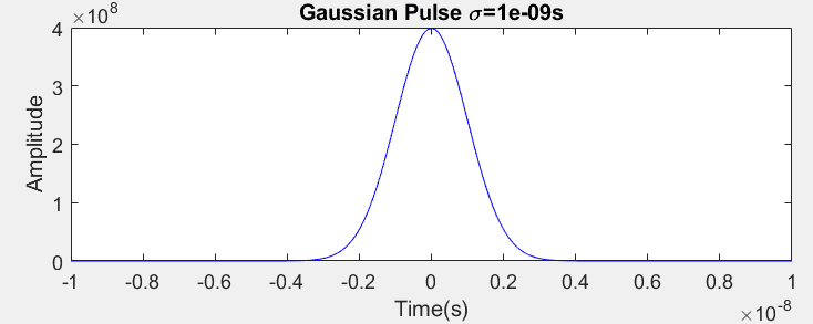
1638757460650.png
 
Last edited:
Physics news on Phys.org
Baluncore said:
Am I right in thinking the graphed function has a FWHM of about 2.7 ns ?
Yes, I was just trying to supply an example guassian. The derived formula for FWHM is as follows, which you can solve for ##\sigma##.
$$FWHM = 2\sqrt{2ln(2)}\sigma$$
 
Maybe you are including sigma in the square root of one or both equations.
Move sigma from the tail to the head.
FWHM = sigma * 2 * Sqr( 2 * Log( 2 ) )
V(t) = Exp( -0.5 * ( t / sigma)^2 ) / ( sigma * Sqr( 2 * Pi ) )
FWHM = 1 nsec
sigma = 4.2466e-10
t= -0.5 ns; v = 469718639.350
t = 0; max v = 939437278.700
t= +0.5 ns; v = 469718639.350
 
Last edited: