Principal component analysis (PCA) coefficients

[roam]

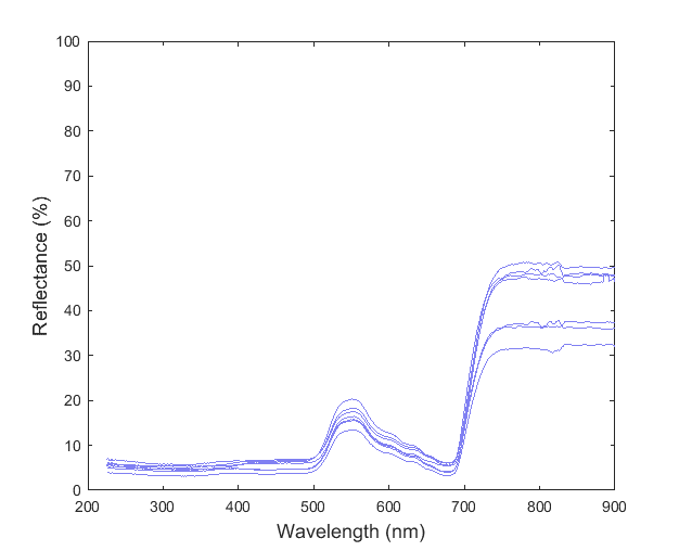
I am trying to use PCA to classify various spectra. I measured several samples to get an estimate of the population standard deviation (here I've shown only 7 measurements):

I combined all these data into a matrix where each measurement corresponded to a column. I then used the pca(...) function in Matlab to find the component coefficients. In this case, Matlab returned 6 components (not a significant dimension reduction since I had 7 measurements).

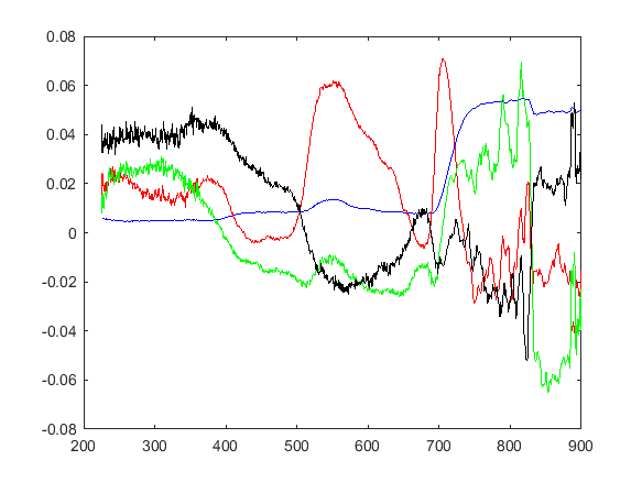
I plotted the first four sets of the component coefficients:

I am not sure how to interpret these curves. The blue curve is the first order coefficients and it resembles the overall shape of the measurement curves. The red curve is the second order coefficient set and it seems to accurately model the shape of the peak at 550 nm (but I don't understand the rest of the curve). The higher order coefficient sets were much noisier.

So, what do these curves represent exactly? Is it possible that each curve is influenced more by the presence of certain components (e.g. molecules of the substance that created the spectrum)?

 

[FactChecker]

A major complication of PCA is that the components can be difficult (or impossible) to interpret in engineering terms. If you can interpret the most significant one, you are doing good. But it sounds like you have not really interpreted the most significant one (the blue line) as you have noticed that it mimics the general shape of the data. That is what the principle component is supposed to do, so it should not be a surprise. That observation is of more value if the shape of the blue line does a better job of fitting a theory of that subject. Then you can look for other subject-dependent explanations of the other lines and arrive at a more detailed theory. That is all up to the subject matter expert and is not a statistical question. Perhaps some experts in spectra can give you some ideas if you supply more detail of where the data came from.

 

[Stephen Tashi]

I plotted the first four sets of the component coefficients:

I don't know what terminology Matlab uses, but I would say you plotted the first four "principal components."

I am not sure how to interpret these curves.

What , if anything, they mean physically is a matter of physics. As a mathematical model it means that the reflectance curves of substances in the population of substances that are tested can be "encoded" by labeling each substance with a set set of coefficients. The decoding of this notation is that the the coefficients c1, c2, c3,..c7 are understood to represent the reflectance curve f = c1 v1 + c2 v2 + ... c7 v7, where the v1, v2,...v7 are a given set of functions of wavelengths (i.e. these functions are the principal components). Furthermore the functions v1, v2,..v7 are chosen and ordered so that (over the population of substances) we have, in a manner of speaking, an efficient system of labeling with respect to losing some of the higher indexed labels. For example, if we only know that the label of a substance begins c1,c2,c3, then our system does the best possible job of approximating f as c1 v1 + c2 v2 + c3 v3, where "best possible job" considers how the system performs over the whole population of substances tested.

You can think of PCA as a method of data compression.

To plot "the component coefficients" of 7 substances, you can plot 7 curves. Each curve will have 7 points on it of the form (k, ck). Wavelength values won't be represented on this graph.

Whether this relates to physics probably hinges on whether the phenomena can be modeled by a superposition of functions. A poetic description of PCA (and ICA and many other statistical techniques) is that they model a result as a "combined effect" of variables. However, the terminology "combined effect" is does not emphasize that PCA and similar techniques model the "combined effect" as an arithmetic sum. An arithmetic sum of variables is very special way to model a combined effect. If there is a physical situation where "adding" things to a system involves all sorts of interactions among the things, then it will be surprising (but not impossible) if the combined effect of some property of the system is the arithmetic sum of certain properties of the things added.

 

[roam]

Hi Stephen Tashi,

My data were spectrophotometer traces of leaves of a given plant species. I want to know if two different species can be distinguished from each other based on their reflectance. But most green plants have a very similar spectrum, for instance, for two different species I found:

Do you think PCA can be useful in pinpointing key differences in a given species that will help identify it from another species?

An arithmetic sum of variables is very special way to model a combined effect. If there is a physical situation where "adding" things to a system involves all sorts of interactions among the things, then it will be surprising (but not impossible) if the combined effect of some property of the system is the arithmetic sum of certain properties of the things added.

In this case, what is considered the "variables"? Is it the chemical constituents, or the wavelengths over which the measurements were taken? As I understand it, the original variables are supposed to be interrelated. PCA transforms into a new set of variables, the principal components, which are then uncorrelated.

Also, the spectrum of a leaf is mainly a linear superposition of the spectrum of chlorophyll, water, and dry matter.

To plot "the component coefficients" of 7 substances, you can plot 7 curves. Each curve will have 7 points on it of the form (k, ck). Wavelength values won't be represented on this graph.

That's right. Matlab's pca function returned a 1350x7 matrix (1350 being the number of wavelengths), and I plotted the first 4 of the 7 rows. So, I believe this corresponds to the principal components.

 

[FactChecker]

IMHO, PCA may not be the best approach. There are advances in neural networks and Artificial Intelegence that are probably better. In fact, they now have facial recognition and identification methods that are pritty good. That seems like the type of methodology that would apply to your problem. I do not have expertise in that area, so that is about all I can say.

 

[Stephen Tashi]

Do you think PCA can be useful in pinpointing key differences in a given species that will help identify it from another species?

I don't know. To investigate this graphically, you need to look a graphs of the coefficents of the principal components and NOT graphs of the principal component functions themselves. The same functions (principal components) are used in making the description of each species, so graphing those functions doesn't tell you anything about how well the descriptions can distinguish species.

If you graph the coefficents of the principal components of a species, the x-axis won't be 200 nm, 300 nm, ... etc. The x-axis will just be 1st, 2nd, 3rd,...etc. It's best to think about the coefficents of a given species as a point in k-dimensional space where k is the number of coefficients we will use in classifying species. The geometric question is whether these points are easily separated from each other by some algorithm or whether they are all bunched up together.

In this case, what is considered the "variables"? Is it the chemical constituents, or the wavelengths over which the measurements were taken?

Your PCA treats each wavelength as a separate variable. It doesn't explicitly model any function that relates the variables.

For example, suppose we have a 20-item rating system for people. The items are things like : sense-of-humor, religious fervor, honesty, shyness,..etc. Applying PCA to these measurements doesn't explicitly model any function that relates (for example) the rating for honesty to the rating for religious fervor. PCA does, in a manner of speaking, account for any linear relation between those two qualities that emerges just from statistics of the population.

For example, there is nothing in the PCA that enforces the idea: Reflectance is a smooth function of wavelength, so the reflectance of a given sample at 350 nm will be close to its reflectance at 300 nm.

As I understand it, the original variables are supposed to be interrelated. PCA transforms into a new set of variables, the principal components, which are then uncorrelated.

Most ideas of "correlation" have to do with a probability model. I think your statement is correct if the probability model is "pick a leaf that was tested at random from the population of those tested".

There is a different type of analysis called Independent Component Analysis (ICA), whose goal is to find a way to generate a joint distribution as the distribution of the sum of independent random variables.

 

[roam]

Hi Stephen Tashi,

I don't know. To investigate this graphically, you need to look a graphs of the coefficents of the principal components and NOT graphs of the principal component functions themselves. The same functions (principal components) are used in making the description of each species, so graphing those functions doesn't tell you anything about how well the descriptions can distinguish species.

If you graph the coefficents of the principal components of a species, the x-axis won't be 200 nm, 300 nm, ... etc. The x-axis will just be 1st, 2nd, 3rd,...etc. It's best to think about the coefficents of a given species as a point in k-dimensional space where k is the number of coefficients we will use in classifying species. The geometric question is whether these points are easily separated from each other by some algorithm or whether they are all bunched up together.

Could you please explain this a bit more? If I understand it correctly, what you are suggesting is to make a 1-D graph (the value of the coefficients against their order). Or are you suggesting something like "biplots"?

Also, to make sure I understood this correctly:

If $p$ is the number of observations and there are $n$ variables/wavelengths ($n \gg p$), in PCA each of the reflectance observations will be represented by linear functions:

$$c_{1}^{\prime}v=c_{11}v_{1}+v_{12}v_{2}+...+c_{1p}x_{p}=\sum_{j=1}^{p}c_{1j}v_{j}$$
$$\vdots$$
$$c_{p}^{\prime}v=c_{p1}v_{1}+v_{p2}v_{2}+...+c_{pp}x_{p}=\sum_{j=1}^{p}c_{pj}v_{j}$$

It therefore reduces the dimension from $n\times p$ to $p\times p$. This means that up to $p$ PCs could be found. So, the way we reduce the dimensionality of the data further is to choose some $m\ll p$ for the number of PCs to keep. In other words, we discard some of the higher order PCs by assuming that most of the variation in the population is accounted for by $m$ PCs, and the higher order ones mostly model noise. Is this correct?

Is it then possible to argue that the higher order principal components would not be very useful for distinguishing between two species?

IMHO, PCA may not be the best approach. There are advances in neural networks and Artificial Intelegence that are probably better. In fact, they now have facial recognition and identification methods that are pritty good. That seems like the type of methodology that would apply to your problem. I do not have expertise in that area, so that is about all I can say.

Noted. PCA might not be the best way to deal with this problem. But I am looking for the simplest way to analyze the spectra, and I think we should still be able to use the more classical techniques to establish if there are discernible differences between the two species.

 

[Stephen Tashi]

Could you please explain this a bit more? If I understand it correctly, what you are suggesting is to make a 1-D graph (the value of the coefficients against their order). Or are you suggesting something like "biplots"?

I'm not familiar with biplots or "1-D graphs", but yes, I am suggesting that you make some sort of graphical representation that shows the coefficients of each species - or at least the coefficients of the first few principal components. (perhaps "spider graphs"?).

If $p$ is the number of observations and there are $n$ variables/wavelengths ($n \gg p$), in PCA each of the reflectance observations will be represented by linear functions:

I don't understand what the "'" signifies in your notation. The main ideas can be understood without writing summations over the $n$ wavelengths.If we have measurements at each of $n$ wavelengths then each principal component can be regarded as one n-dimensional vector.

Suppose we have $k$ individual leaves that are measured at each of those wavelengths. The results of a test of one those things is also represented as one n-dimensional vector.

Let $w_1,w_2,...w_k$ be k vectors, each of which is a result of a test.
Let $v_1, v_2,...v_k$ be (as yet unspecified) n-dimensional vectors.

It is obvious that we can express each $w_j$ in a trivial manner by setting:
$v_j = w_j$ and writing
$w_j = \sum_{i=1}^k c_{j,i} v_i$ with $c_{j,j} = 1$ and the other $c_{j,*}$'s = 0. This just says $w_j$ is equal to itself.
Also, in a trivial sense, it is easy to distinguish the $w_*$'s using their coefficients. For example the coefficients for $w_1$ are (1,0,0,...0), the coefficients for $w_2$ are $(0,1,0,0,...)$ etc.

If we apply PCA, we get a different set of vectors (functions) $v_1, v_2,...v_k$ that are no longer identical to the $w_*$'s. We find different coefficients for each $w_j$ such that $w_j = \sum_{i=1}^k c_{j,i} v_i$ Distinguishing the $w$'s by their coefficients is no longer trivial. For example, $w_1$ might have coefficients like (0.79, -0.32, 4.61,...).

We get "dimension reduction" if we can approximate each $w_j$ by using only the first few principal components. For example, suppose 3 < k and that the approximations $w_j \approx \sum_{i=1}^3 c_{j,i} v_i$ are each good for $j = 1,2,..k$.

Dimension reduction is only useful for the purposes of classification if we can find a method to classify the data given by the smaller set of coefficents. For example for the case of 3 coefficients, the result of each test can be represented by a point in 3-dimensional space. There are various techniques for trying to classify such data. "Cluster analysis" is often useful.

Dimension reduction, by itself, does not automatically solve the classification problem. Dimension reduction only reduces the complexity of the data that we attempt to classify.

I have avoided writing sums over the index of the $n$ wavelengths by talking in terms of vectors. Of course, if you want to write-out the component-by-component meaning of $w_j \approx \sum_{i=1}^k c_{j,i} v_i$, it would be (for the $s$-th component, $s = 1,2,..n$)
$w_{(j,s)} \approx \sum_{i=1}^3 c_{j,i} v_{(i,s)}$.

 

[roam]

Thank you very much for the explanation.

Dimension reduction is only useful for the purposes of classification if we can find a method to classify the data given by the smaller set of coefficents. For example for the case of 3 coefficients, the result of each test can be represented by a point in 3-dimensional space. There are various techniques for trying to classify such data. "Cluster analysis" is often useful.

Dimension reduction, by itself, does not automatically solve the classification problem. Dimension reduction only reduces the complexity of the data that we attempt to classify.

Is it not more computationally efficient to perform cluster analysis directly on the original data?

Suppose that we are trying to classify based on a feature such as the Euclidean distance between the observations in the original k-dimensional space. Using the first few PCs simply provides an approximation to the original distance that we want to use for classification. So, doesn't the extra calculation involved in finding the PCs outweigh any savings we get from using $m \ll k$ instead of $k$ variables?

Another question that I have, is whether I should be looking into "cluster analysis" or "discriminant analysis"?

In my situation, I have a large number of leaf measurements ($w_1, ... , w_k$) for which the group membership of each observation is already known. The aim is to use this data as a kind of "training set" so that future measurements can be automatically classified.

Also, would PCA be useful in a discriminant analysis (i.e. if we only use the first few PCs in the derivation of the discriminant rule)?

I don't understand what the "'" signifies in your notation. The main ideas can be understood without writing summations over the $n$ wavelengths.

The " ' " denotes transpose. The formula I used is from the textbook "Principal Component Analysis" by Jolliffe, but I think your formulation is clearer.

 

[Stephen Tashi]

Is it not more computationally efficient to perform cluster analysis directly on the original data?

Are you comparing it to using all the principal components? If you use all the principal components then, yes, you are effectively doing cluster analysis on the original data with the added burden of expressing the data in PCA. However, using on a few of the principal components need not give you the same results as a cluster analysis on the original data - which may be good if the higher order principal components are due to "noise" of some sort (errors in measurement, variability of different specimens of the same species).

Another question that I have, is whether I should be looking into "cluster analysis" or "discriminant analysis"?

I don't know much about discriminant analysis. To me, typical neural nets are a form of non-linear discriminant analysis. They perform a non-linear mapping of the data points to other points in space and then a response node defines a plane that separates the data. By doing compositions of these non-linear mappings, you effectively define non-linear boundaries around volumes in the original data.

In my situation, I have a large number of leaf measurements ($w_1, ... , w_k$) for which the group membership of each observation is already known. The aim is to use this data as a kind of "training set" so that future measurements can be automatically classified.

My advice is to first characterize the variability of each species. For each species, find a good probability model for the response curve of a randomly selected leaf of that species. If you are doing research in botany, this gets you closer to the science of leaves. Of course, if you are doing a project for a course in data analysis, the evaluators may be more interested in seeing statistical techniques than botanical science.

I'm not a botanist, but if I were collecting spectral response data from a fragment of a leaf, I'd measure it and then move the specimen a little to see how much the measurement changed. I'd flip the specimen over and measure it from the other side. Those type of measurements characterize the variability of response in a single leaf. Then one can investigate variability among different leaves on the same plant and plant-to-plant differences in the same species.

 

[WWGD]

Hi Stephen Tashi,

My data were spectrophotometer traces of leaves of a given plant species. I want to know if two different species can be distinguished from each other based on their reflectance. But most green plants have a very similar spectrum, for instance, for two different species I found:

View attachment 234797
Also, the spectrum of a leaf is mainly a linear superposition of the spectrum of chlorophyll, water, and dry matter.
.

Can't you build your PC A around this ?

 

[roam]

Are you comparing it to using all the principal components? If you use all the principal components then, yes, you are effectively doing cluster analysis on the original data with the added burden of expressing the data in PCA. However, using on a few of the principal components need not give you the same results as a cluster analysis on the original data - which may be good if the higher order principal components are due to "noise" of some sort (errors in measurement, variability of different specimens of the same species).

Thanks a lot for the explanation.

My advice is to first characterize the variability of each species. For each species, find a good probability model for the response curve of a randomly selected leaf of that species.

Do you mean that I should collect additional measurements? At the present, I have about 30 leaf measurements for each species, and that gives the standard deviation bounds shown in post #4. I know that I would need well over 100 measurements to have a statistically meaningful standard deviation estimate. But realistically I can't collect such a large data set (I wonder if there is a rule of thumb for when you could stop collecting further measurements).

Also, would you say that the regions with complete overlap (e.g. 750–900 nm in my post #4) are useless for classifications?

I'm not a botanist, but if I were collecting spectral response data from a fragment of a leaf, I'd measure it and then move the specimen a little to see how much the measurement changed. I'd flip the specimen over and measure it from the other side. Those type of measurements characterize the variability of response in a single leaf. Then one can investigate variability among different leaves on the same plant and plant-to-plant differences in the same species.

My project is in applied physics and it does relate to botany. A part of the project involves using remote sensing to delineate certain plant species from the crops. Based on my data, I don't know yet if it is feasible to positively classify a given measurement. We will be imaging the plants from above, so all of my measurements are from the upper (adaxial) surface of the leaf lamina. For all specimens, I measured the same location which was the meristem (a small young leaf in the center of the plant, or the growing point).

Suppose we have 3 species: species A, species B, and the crops. I am looking for a way to measure the degree to which species A is more discernible from the crops than species B.

If I retain a subset of the principal components (the first few high variance PCs) and exclude higher order ones that are likely contaminated by noise, do you think that could be plotted to give a good graphical representation of the degree of dissimilarity between two species? I mean, we could plot the first few PCs for each species separately (e.g. on spider graphs) and then compare the plots. Could this be used as a way to show how good, or otherwise, the separation between the groups are?

Can't you build your PC A around this ?

What do you mean exactly? I am trying to use PCA on both data sets...

 

[Stephen Tashi]

I know that I would need well over 100 measurements to have a statistically meaningful standard deviation estimate.

Suppose we have 3 species: species A, species B, and the crops. I am looking for a way to measure the degree to which species A is more discernible from the crops than species B.

Neither "standard deviation" nor "degree" of discernability has a specific meaning until we define specific random variables and attempt a specific procedure.

If I retain a subset of the principal components (the first few high variance PCs) and exclude higher order ones that are likely contaminated by noise, do you think that could be plotted to give a good graphical representation of the degree of dissimilarity between two species? I mean, we could plot the first few PCs for each species separately (e.g. on spider graphs) and then compare the plots. Could this be used as a way to show how good, or otherwise, the separation between the groups are?

Yes I think you should attempt to do this, but I can't know in advance whether it will be a successful procedure.

Concerning your previous comment:

Also, the spectrum of a leaf is mainly a linear superposition of the spectrum of chlorophyll, water, and dry matter.

You could pursue @WWGD 's suggestion in the following manner.
Let the spectral response curves of chlororphyl, water, and dry matter be, resectively $C(\lambda), W(\lambda),D(\lambda)$.
Let $F(\lambda)$ be the spectral response curve of a given leaf.
Assume $F(\lambda) = x\ C(\lambda) + y\ W(\lambda) + z\ W(\lambda)$ where $x,y,z$ are constants.

Solving for $x,y,z$ requires solving an overdetermined system of $N$ linear equations where $N$ is the number of wavelengths at which a response measurement is taken. For each wavelength $\lambda_i$ we have the linear equation
$F(\lambda_i) = x\ C(\lambda_i)+ y\ W(\lambda_i) + z\ W(\lambda_i)$.

An over determined system of linear equations can be solved "in the least squares sense". So for each leaf you can get values of $x,y,z$. If the relative contribution of chlorophyll, water, and dry matter is a distinguishing feature of a species, you could classify the species by their $x,y,z$ values. It's a matter of biology whether different leaves have distinguishing proportions of chlorophyll, water and dry matter. You might be able to measure those proportions in a laboratory to check your estimates of $x,y,z$.

 

[FactChecker]

If I retain a subset of the principal components (the first few high variance PCs) and exclude higher order ones that are likely contaminated by noise, do you think that could be plotted to give a good graphical representation of the degree of dissimilarity between two species?

I think this is wrong. The principle components might be the best representation of the common aspects of both types. You are looking for the differences, not the common aspects. And the noise might be associated the principle components more than the less significant components and contaminate them more. IMHO, you should start by doing a multiple linear stepwise regression of the type based on the other variables and see what the result is and how statistically significant it is as a predictor of type. The stepwise regression process should identify the combination of variables that best distinguishes between types.

 

[roam]

Hi Stephen Tashi,

I managed to plot the observations for two species with respect to their first two PCs. For one species I had 25 measurements (shown in blue), and for the other species I had 10 specimen measurements (red). Assuming that my computations were correct, here is what I got:

Close-up:

If I draw a convex hull around each species, the red species will be completely encompassed by the blue. Does this mean that we cannot differentiate the two species from each other?

When I tried to plot PC3 against PC1, the results were the same. In fact, according to Matlab, PC1, PC2, and PC3, respectively account for 99.8%, 0.0829%, and 0.0255% of the variation. I am not sure how to interpret that. But the percentage of total variation is a measure of how good the 2D representation is, so I think a higher dimension plot would not be very helpful.

Also, why do I get an extreme outlier for each set (as shown in the first picture above)? My spectrophotometric traces were all fairly close to each other — for instance, for the blue species I had:

You could pursue @WWGD 's suggestion in the following manner.
Let the spectral response curve

s of chlororphyl, water, and dry matter be, resectively $C(\lambda), W(\lambda),D(\lambda)$.
Let $F(\lambda)$ be the spectral response curve of a given leaf.
Assume $F(\lambda) = x\ C(\lambda) + y\ W(\lambda) + z\ W(\lambda)$ where $x,y,z$ are constants.

Solving for $x,y,z$ requires solving an overdetermined system of $N$ linear equations where $N$ is the number of wavelengths at which a response measurement is taken. For each wavelength $\lambda_i$ we have the linear equation
$F(\lambda_i) = x\ C(\lambda_i)+ y\ W(\lambda_i) + z\ W(\lambda_i)$.

An over determined system of linear equations can be solved "in the least squares sense". So for each leaf you can get values of $x,y,z$. If the relative contribution of chlorophyll, water, and dry matter is a distinguishing feature of a species, you could classify the species by their $x,y,z$ values. It's a matter of biology whether different leaves have distinguishing proportions of chlorophyll, water and dry matter. You might be able to measure those proportions in a laboratory to check your estimates of $x,y,z$.

Unfortunately, I can't measure the proportions of the biochemical constituents individually. I can only measure the total signal from intact leaves (here is my setup).

So, basically, we can assume that $C(\lambda), W(\lambda),D(\lambda)$ are the first 3 principal components?

In the spectral region that I am looking at, the spectrum is largely due to chlorophyll. Water and dry matter play a comparatively small role. If PC1 accounts 99.8%, then it could likely be related to chlorophyll. But "chlrophyll" is itself composed of several different types of pigments whose concentrations vary from plant-to-plant. I guess $C(\lambda)$ cannot be broken down further into those individual components that make up the chlorophyll?

I think this is wrong. The principle components might be the best representation of the common aspects of both types. You are looking for the differences, not the common aspects. And the noise might be associated the principle components more than the less significant components and contaminate them more. IMHO, you should start by doing a multiple linear stepwise regression of the type based on the other variables and see what the result is and how statistically significant it is as a predictor of type. The stepwise regression process should identify the combination of variables that best distinguishes between types.

Thanks a lot for the suggestion. I will definitely be looking into that. But I think we should be able to judge the degree of similarity by looking at the areas of a 2D plot covered by various subsets of observations. These kinds of diagrams could be a very simple way of delimiting the species.

 

[roam]

I had made a mistake. Here is what my results should look like:

$$
\begin{array}{c|c|c}
& \text{PC} & \text{Percentage}\\
\hline & 1 & 91.1\\
\text{Species 1} & 2 & 7.9\\
& 3 & 0.7\\
\hline & 1 & 96.2\\
\text{Species 2} & 2 & 2.7\\
& 3 & 0.6
\end{array}
$$

From these results, what can we say about the discernibility of the two species?

Also, I didn't understand how the PCs relate to each of the three functions in the linear sums:

$x C(\lambda)+y W(\lambda)+z D(\lambda).$

Any explanation would be appreciated.

 

[FactChecker]

You can see the problem with using PCs here. PC#1 is the best single representation of BOTH species (91% and 96%), so it is not clear how to use it to distinguish between species. This is the wrong approach. You need an approach that is specifically designed to distinguish between the species. That is what a linear regression of species based on the other variables would do. I think that your desire to use PCs is misleading you here.

But I think we should be able to judge the degree of similarity by looking at the areas of a 2D plot covered by various subsets of observations. These kinds of diagrams could be a very simple way of delimiting the species.

I want to know if two different species can be distinguished from each other based on their reflectance.

You are not looking for similarities, either within species or overall. You are looking for differences so that you can distinguish between the species. That is a very different problem.

 

[Stephen Tashi]

So, basically, we can assume that $C(\lambda), W(\lambda),D(\lambda)$ are the first 3 principal components?

No, you can't assume that. Fundamental mathematical things sometimes correspond to fundamental physical things, but this doesn't always happen.

There are various ways to represent a response function as a linear combination of other functions. For example, if you were in the field of signal processing, you would naturally express a response function as a Fourier series. You an also express functions in various ways using various sets of "orthogonal polynomials".

The functions $C(\lambda), W(\lambda), D(\lambda)$ are probably not orthogonal functions. For example, suppose you want to express a response function $R(\lambda)$ as the sum of orthogonal and orthonormal functions and you want to know the coefficent for the 3rd orthonormal function $f_3(\lambda)$ in that set. You can find the coefficient by computing $c_3 = \sum_{\lambda \in \Lambda} R(\lambda)f_7(\lambda)$.

By contrast, the problem of expressing $R$ as a linear combination of $C(\lambda),W(\lambda),D(\lambda)$ may have more than 1 possible answer for the coefficients or no answer at all. Then you need to add more conditions to the problem (such as best least square fit) to specify a unique result. However, since $C,W,D$ have some physical interpretation, using those functions might (or might not!) provide insight in the physics.

As @FactChecker indicates, your problem is not one of "cluster detection". Instead, you already know the clusters you want - namely you want a cluster at each individual plant species. Your problem is to find a representation of the data plus a method of cluster detection that reproduces the desired clusters when applied to that representation.

The best practical way to investigate this problem depends on your skills with computer software. For example, you might be a sophisticated programmer (or have the use of one) or you might only be comfortable with using particular software programs.

 

[roam]

Hi @Stephen Tashi,

I have a follow-up question. I have found a paper which shows that the concentrations of the components $C\left(\lambda\right),\ W\left(\lambda\right)$ and $D\left(\lambda\right)$ are are not statistically independent and co-vary. Does this fact mean that PCA will be unable to resolve the principal components along the lines of the actual physical components? (principal components are supposed to be uncorrelated)

To clarify: the paper is really talking about the correlations between the concentration (e.g. μg/cm²) of the components. I think this corresponds to the constants, $x,\ y$, and $z$ in your post #13, which are the coefficients of the PCA. It doesn't mean that the actual functions $C,\ W, \ D$ are themselves correlated (indeed the reflectance of the three substances are entirely different).

 

[Stephen Tashi]

To clarify: the paper is really talking about the correlations between the concentration (e.g. μg/cm²) of the components. I think this corresponds to the constants, $x,\ y$, and $z$ in your post #13, which are the coefficients of the PCA.

I don't know what you mean by "this". It's also unclear what "correlation" means until we have specified what random variables are involved. For example, how do you define the concentration of chlorophyll or the concentration of water as random variables? One thought is that we pick a plant at random from the population of plants and measure the concentrations of the substances in the plant.

With that interpretation, the $x,y,z$ of post 13 can be considered as random variables. These random variables are not coefficients of the principal components because $C,W,D$ are (probably) not the principal components.

It doesn't mean that the actual functions $C,\ W, \ D$ are themselves correlated (indeed the reflectance of the three substances are entirely different).

What would it mean to say two functions are "correlated"? or "uncorrelated"? We can speak of functions ( and vectors) as being "linearly independent". The "independence" of 3 functions is a geometric idea, not a statistical idea. To say $C(\lambda),W(\lambda),D(\lambda)$ are linearly independent means you can't express one function as a linear combination of the other two functions. "independence" of functions is a different concept that "uncorrelated-ness" of random variables.

For example, the functions $f(\lambda) = \lambda^2 + 2\lambda, \ g(\lambda) = 4\lambda, \ h(\lambda) = 3\lambda^2 + \lambda$ are not a linearly independent set because $h = 3f - (5/4) g$

A stronger property than "independence" is the property of "orthogonal". Two 3-dimensional vectors can be orthgonal, and, similarly, two functions can be orthogonal when considered as many dimensional vectors.

 

[roam]

Thanks a lot for the explanation. Yes, I meant something similar to "linearly independent" or "orthogonal". The shapes of the reflectance curves for those substances are completely unrelated because the molecules or chromophores that generate them are entirely different.

Yet, the amount of these substances present in a given leaf seem to be statistically related (i.e. they co-vary in nature). For instance, from literature we can find this kind of correlations between the concentration of components:

I don't know what you mean by "this".

In post #13 you said that the constants $x, \ y, \ z$ relate to the "relative contribution a given component", which relates to the concentration of the given substance. Based on what we saw in literature, these constants are statistically correlated. I was wondering if this correlation has anything to do with the fact that PCA cannot isolate $C,W,D$ as the principal components?

It's also unclear what "correlation" means until we have specified what random variables are involved. For example, how do you define the concentration of chlorophyll or the concentration of water as random variables? One thought is that we pick a plant at random from the population of plants and measure the concentrations of the substances in the plant.

With that interpretation, the $x,y,z$ of post 13 can be considered as random variables. These random variables are not coefficients of the principal components because $C,W,D$ are (probably) not the principal components.

Yes, that's true. I was talking hypothetically, assuming that $C,W,D$ were the principal components.

But we already know that the principal components are not $C,W,D$ because when I plot the PC loadings against wavelength (as in post #1), none of the curves resemble the reflectance curves of pure water, pure chlorophyll, etc. That makes it very difficult to interpret the PCs physically.

The exception is the curve for the first PC; it resembles a complete reflectance measurement of a given leaf. Is it then possible to interpret PC1 as the "overall reflectance"? In textbooks, I have seen PCA examples where the variables are various anatomical measurements of individuals, and they interpret the first PC (accounting for a large proportion of the total variation) as the "overall size" of each individual.

 

[Stephen Tashi]

The exception is the curve for the first PC; it resembles a complete reflectance measurement of a given leaf.

That might be remarkable , depending on how you applied PCA to the data.

This following is the way I think of it.

We agree the "distance" between two reflectance curves $f(\lambda)$, $g(\lambda)$ is to be measured by
$D(f,g) = \sqrt{ \sum_{\lambda \in\Lambda}(f(\lambda) - g(\lambda))^2}$

For a set of $S$ of $N$ reflectance curves, we define the "average curve" to be $m(\lambda) = (1/N) \sum_{f \in S} f(\lambda)$.

It isn't surprising that the average reflectance curve resembles a typical reflectance curve.

We now pose the problem of how "best" to approximate each curve $f$ in the set $S$ as

$f(\lambda) \approx m(\lambda) + A_f p_1(\lambda)$

where $p_1(\lambda)$ is a given function - i.e. we must use the same $p_1$ for each $f$
and $A_f$ is a number that can be different for different $f$. Once $p_1$ is specified, we agree that $A_f$ will be the number that minimizes
$D(f,\ m(\lambda) + A_f p_1(\lambda))$.

We define what it means for $p_1$ to be the "best" curve by requiring that $p_1$ be the curve that minimizes the average distance of curves from their approximations - i.e. $p_1$ minimizes $(1/N) \sum_{f \in S} D(f, \ m + A_f p_1)$.

(A poetic way people describe $p_1$ is that it best explains the variability of the the curves. However, to me, it is the various constants $A_f$ that "explain" the variability of the curves insofar as they "explain" or implement the distinction among the approximations. I'd say that $p_1$ is the curve that best allows the associated $A_f$'s to explain how the curves vary from the average curve. )

From the above point of view, I see no reason that the curve $p_1$ should resemble a typical reflectance curve. Perhaps there is some confusion in how your software denotes $m(\lambda)$ versus the first principal component $p_1$?

 

[roam]

From the above point of view, I see no reason that the curve $p_1$ should resemble a typical reflectance curve. Perhaps there is some confusion in how your software denotes $m(\lambda)$ versus the first principal component $p_1$?

Yes, that's very strange. But I am sure what I plotted is meant to be PC1 not the mean $m(\lambda)$ . I plotted the columns of the loading matrix for each of the PCs, so the first column corresponds to the first PC, etc.

However, I conducted the PCA on the covariance matrix, rather than on the correlation matrix of the variables (the software allows both methods).

Also in my data, the standard deviation varied a lot among the variables (e.g. being very small in the blue, and very large in the green region of the spectrum). Jolliffe's textbook says that in such situations you have to apply PCA on the correlation matrix:

"...using a covariance matrix to find PCs when the variables have widely differing variances; the first few PCs will usually contain little information apart from the relative sizes of variances, information which is available without a PCA."

Now when I applied PCA to the correlation matrix instead, PC1 no longer resembles a typical reflectance curve. Here is a comparison (covariance matrix on the left, and correlation matrix on the right):

So, how exactly does using the covariance matrix influence PC1 to resemble a typical reflectance measurement?

 

[Stephen Tashi]

So, how exactly does using the covariance matrix influence PC1 to resemble a typical reflectance measurement?

I can only spin a tale inexactly.

Using the notation from post 22 , if you use the correlation matrix, you are changing the problem from that of trying to best estimate functions $f(\lambda)$ to the problem of trying to estimate a different set of functions that are "normalized" versions of the $f(\lambda)$

For each wavelength $\lambda$, consider the set of values $\{f(\lambda):f \in S\}$ Compute the sample mean $\mu_{\lambda}$ and sample standard deviation $\sigma_\lambda$ of those values. For each function $f(\lambda)$ define a new function $z_f(\lambda) = ( f(\lambda) - \mu_\lambda)/ \sigma_\lambda$. Using the correlation matrix from the data is equivalent to the problem of finding a set of principal components that are best for estimating the functions $z_f$.

Instead of taking the view that the purpose of $p_1(\lambda)$ is to estimate the functions in $S$, now take the view that goal of $p_1(\lambda)$ is to create a linear combination $L_1(f) = \sum_{\lambda \in \Lambda} p_1(\lambda) f(\lambda)$ that has maximum variance as $f$ ranges over the functions in $S$, subject to some constraint on the values of $p_1(\lambda)$, such as $\sum_{\lambda \in \Lambda} p_1(\lambda)^2 = 1$.

I don't have a good intuitive argument about why the "maximize variance" approach to $p_1$ is equivalent to the "best estimate" approach. I've just heard both approaches used so often that I accept they are equivalent.

A particular feature of your data is that values of $\lambda$ whose $f(\lambda)$ are small also have small variances in the $f(\lambda)$. In fact, a rough approximation might be $\sigma_\lambda = k \mu_\lambda$ i.e. $\sigma_\lambda = k m(\lambda)$ for some constant $k$ that is the same for all $\lambda$.

By contrast, for the scaled values given by the $z_f(\lambda)$, the variance of the values in the set $\{z_f(\lambda): f \in S\}$ is 1 for each given $\lambda$

If we are trying to create a $L_1(z_f) = \sum_{\lambda \in \Lambda} p_1(\lambda)z_f(\lambda)$ that has maximum variance, then no value of $\lambda$ has an a priori greater significance than any other value as far as variance goes because all sets $\{ z_f(\lambda):f \in S \}$ have the same variance. So there is no reason to expect that the shape of the function $p_1(\lambda)$ will have a definite relation to the shape of $\sigma_\lambda = k m(\lambda)$.

On the other hand, if we are trying to create an $L_1(f)$ that has maximum variance then it makes some intuitive sense that $p_1(\lambda)$ should be larger for values of $\lambda$ whose $f(\lambda)$ have larger variances. to "give more weight" to them. In your data this amounts to $p_1(\lambda)$ being large when $k m(\lambda)$ is large. So a hasty intuition can accept that the shape $p_1(\lambda)$ resembles the shape of $m(\lambda)$

If we try to add logic to naive intuition, we get into complexities. Why not pick the $\lambda_0$ such that the variance of the set $\{f(\lambda_0):f \in S\}$ is the largest possible and then set $p(\lambda_0) = 1$ and the rest of the $p(\lambda) = 0$ ? That would work if the sets $\{f(\lambda):f \in S\}$ were independent of each other for values of $\lambda$. However, they are not. They occur from a common $f$. Why doesn't this dependence destroy any relation between the shape of $p_1$ and the shape of $m(\lambda)$? I suspect their are data sets where it does destroy it.

That's the limit of my inutition at the moment.

 

[roam]

Thanks a lot for this explanation, I agree with that. I have a related question.

As I mentioned before, my software allows both the use of variance-covariance matrix as well as the correlation matrix. But there is the additional option of performing PCA "within-group" or "between-group".

From what I understand, for the "within-group" option, the average $m$ within each group is subtracted before the eigenanalysis to remove the differences between the groups. In my situation, all green plant populations have spectra that behave very similarly, differing mainly in mean.

I am not sure how exactly the mathematics works for the "between-group" option, but I believe the algorithm uses the group means $m$ instead (the software documentation doesn't really explain the details). It analyzes the groups rather than the individual measurements. It doesn't work when there are only 2 groups because it returns only 1 PC for some reason. When there are 3 groups present, it returns 2 PCs, and so on.

I think I should use the correlation matrix because of the widely varying standard deviations. But I am not sure whether I should use the "between-group" PCA, or disregard the "between/within-group" option. What type of PCA would you think is most appropriate for this data?

 

[FactChecker]

I have not followed a lot of this thread, and do not have the background to understand much of it. For my own curiosity, I wonder why you are trying to use PCA for this problem. My general classification of problems and the appropriate statistical analysis leads me to suggest regression analysis:

Analysis Types:

• Looking for descriptions of similarities of a group: Principle Component Analysis (PCA); Factor Analysis
• Looking for ways to define distinguishable groups (without preconcieved grouping): Cluster analysis
• Looking for explanations and predictors for a known difference: Regression analysis; Analysis of Variance (ANOVA)
  

 

[roam]

Hi @FactChecker,

My spectrophotometric measurements are based on 1350 wavelengths/variables. The aim of my project is to differentiate plants based on a much smaller subset of wavelengths. At the present, I want to know what the most significant variables are. When plotting the results of a PCA, if the separation between two known groups is in terms of a given PC, then plotting the loadings of that PC against variables (as in post #23) tells you what variables are most significant when it comes to distinguishing. The variables for which the loadings are largest in absolute value are the variables where the most important distinguishing features occur (at least that is my understanding). Do you believe I am on the right track?

As I understand it, cluster analysis doesn't really give this information. For instance, the following are the dendrograms I made based on Pearson's correlation on the left and Euclidean distance on the right (by the way, do you know why is the former such a better distance metric for classifying the spectra?). The colours indicate the actual group membership of a measurement.

Do you think regression analysis does a better job of telling you what the best variables are?

 

[FactChecker]

Hi @FactChecker,

My spectrophotometric measurements are based on 1350 wavelengths/variables. The aim of my project is to differentiate plants based on a much smaller subset of wavelengths. At the present, I want to know what the most significant variables are. When plotting the results of a PCA, if the separation between two known groups is in terms of a given PC, then plotting the loadings of that PC against variables (as in post #23) tells you what variables are most significant when it comes to distinguishing. The variables for which the loadings are largest in absolute value are the variables where the most important distinguishing features occur (at least that is my understanding). Do you believe I am on the right track?

As I understand it, cluster analysis doesn't really give this information. For instance, the following are the dendrograms I made based on Pearson's correlation on the left and Euclidean distance on the right (by the way, do you know why is the former such a better distance metric for classifying the spectra?). The colours indicate the actual group membership of a measurement.

View attachment 237294

Do you think regression analysis does a better job of telling you what the best variables are?

IMHO, yes. Stepwise regression analysis (see https://en.wikipedia.org/wiki/Stepwise_regression) is specifically designed to determine the best variables to distinguish between values of a dependent variable. So yes, it is made exactly for that. Your dependent variable can be a 0,1 variable which indicates the plant type. A forward stepwise regression would start with the single variable (wavelength) that does the most to determine the plant type. Then, having accounted for the first variable, it would look for the second variable which does the most to add accuracy to the determination. It continues like that till there are no other variables which are statistically worth adding. IMHO, the best version is "bidirectional elimination". After several variables have been added to the model, the early variables may not add much that a combination of the later variables do not already do. If the early variable is no longer statistically significant, the bidirectional elimination algorithm will remove it.

I have assumed that you are looking for the variables that distinguish between two plant types, not more. That allows you to define a 0,1 variable indicating the plant type. If there are more than two plant types which you want to analyze in the same model, that is different and my recommendation would have to be re-evaluated.

 

[Stephen Tashi]

As I mentioned before, my software allows both the use of variance-covariance matrix as well as the correlation matrix. But there is the additional option of performing PCA "within-group" or "between-group".

What software are you using?

 

[roam]

What software are you using?

I was using a free software called PAST (Paleontological Statistics by Hammer et al., 2001).