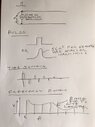
I Pulse bouncing off ends of a tube, expressed as sum of sine modes?

[Swamp Thing]

If we start with an initial y(x, t=0) we can represent the initial profile as a sum of sinusoids, and then sum up the the trivial evolutions of all components - as explained in the video below.

But if we start with a narrow pulse propagating in one direction and bouncing back and forth, is it possible to do the same? If yes, how to calculate the contributions of different sinusoidal modes in this case?

 

[Andy Resnick]

If we start with an initial y(x, t=0) we can represent the initial profile as a sum of sinusoids, and then sum up the the trivial evolutions of all components - as explained in the video below.

But if we start with a narrow pulse propagating in one direction and bouncing back and forth, is it possible to do the same? If yes, how to calculate the contributions of different sinusoidal modes in this case?

The phenomenon you are thinking of is 'group velocity dispersion'.

 

[Swamp Thing]

If we assume non dispersive propagation, can a single back-and-forth bouncing pulse be represented as a sum of sinusoidal standing waves?

If yes, how do we get the coefficients?

If no, then does that prove that a truly non dispersive line is impossible?

 

[Andy Resnick]

If we assume non dispersive propagation, can a single back-and-forth bouncing pulse be represented as a sum of sinusoidal standing waves?

I don't think a traveling wave can be represented by a combination of standing waves unless you allow the amplitudes to be functions of time. That said, I've never really understood mode locking, so I could be mistaken.

 

[Baluncore]

... if we start with a narrow pulse propagating in one direction and bouncing back and forth, is it possible to do the same? If yes, how to calculate the contributions of different sinusoidal modes in this case?

Model the tube as a transmission line, rather than as a string, or a resonator. Oliver Heaviside came up with the "telegrapher's equations", and worked out how to equalise the dispersion of a transmission line. Heaviside was also the first to apply the Dirac delta function.

 

[Swamp Thing]

Model the tube as a transmission line, rather than as a string, or a resonator.

I thought closed tubes and strings were equivalent to transmission lines with open ends (if we make pressure the analog of voltage). But no, the electrical line has a leakage conductivity part besides the series loss, which makes it perhaps more mushy.

But to return to my question, let us assume a "spherical cow" in the form of an ideally non-dispersive tube / string / transmission line.

I don't think a traveling wave can be represented by a combination of standing waves unless you allow the amplitudes to be functions of time.

I was under the impression that any solution of the 1-D wave equation with boundaries at both ends can be represented as a sum of modal oscillations. But now it looks like either (a) only certain solutions can be represented that way, OR (b) the problem arises simply because that particular spherical cow doesn't exist in reality, and the pulse remaining undistorted forever is an impossible thing.

If (a), then how can we classify the initial conditions by inspection without actually solving the thing?

 

[Baluncore]

Frequency dependent dispersion will occur at open tube ends, where the diameter and wavelength interact. For that reason, you need to consider physical tubes with closed ends only.

Your hypothetical narrow pulse is a Dirac delta function, which has a continuous spectrum. But that spectrum will not last. For a fixed length tube, there will be a comb of deep nulls in the spectrum, that arise from cancellation of the same direction reflections. Between those nulls will be the standing waves due to opposite direction summation of the surviving sinusoids.

But no, the electrical line has a leakage conductivity part besides the series loss, which makes it perhaps more mushy.

The real tube is lossy. An ideal electrical transmission line model can be perfect, with zero dispersion.

The propagating sinusoids that survive, and the resonant waveform, could be modelled using SPICE as a perfect lossless transmission line. The ends of the line could be open or closed, but SPICE would not correctly simulate real open-ended tubes.

 

[Swamp Thing]

There is a clue in Prof. Lewin's video in my original post. He looks at a case where he sets up a narrow-ish pulse in the middle of the string and lets it go. The trouble is, this is a symmetrical case: you see two pulses heading off from the middle towards the ends.

My problem was how to synthesise a pulse that somehow knows that it is supposed to move right and not left after release.

The answer is: First pretend that your string / tube / cable is twice as long as it actually is, and set up your pulse in the middle of this 2L line. Then resolve into components and evolve as Lewin explains. But finally, ignore one half of the solution and take one half as the single pulse-in--a-box that you need. The thing is that a pulse bouncing off an end is mathematically equivalent to two pulses overlapping in the middle.

We just focus on one half of the solution in this video...

NB: The plot represents air pressure in a closed tube, or any other analogous problem. In a guitar string, some appropriate substitution of parameter would be required?

 

[Baluncore]

My problem was how to synthesise a pulse that somehow knows that it has to move right and not left after release.

I might inject the pulse as an initial condition, at one end. The energy can then only go one way from there, so it would pass the centre shortly afterwards, going the way you want.

 

[Swamp Thing]

I might inject the pulse as an initial condition, at one end. The energy can then only go one way from there, so it would pass the centre shortly afterwards, going the way you want.

I was not sure if "half a pulse" stuck to the end would work... But come to think of it, it would be like ignoring half of a 2L problem as well. I will try it, thanks.

 

[Swamp Thing]

The Fourier of half a pulse... Truncation issues...?

 

[Swamp Thing]

I might inject the pulse as an initial condition, at one end. The energy can then only go one way from there, so it would pass the centre shortly afterwards, going the way you want.

If you inject a whole pulse just to the right of the left end, it evolves the same as a pulse injected in the middle. It still splits into two pulses, except the left-going pulse bounces almost immediately off the left wall.

If you inject a half pulse momentarily braced against the wall and ready to kick off, its Fourier transform is distorted due to truncation of the time series. (Not that this matters too much for qualitative simulations like what I am trying to do --- in fact it has a more real-world vibe, so rather nice for explanatory demos).

 

[Baluncore]

If you inject a whole pulse just to the right of the left end, it evolves the same as a pulse injected in the middle. It still splits into two pulses, except the left-going pulse bounces almost immediately off the left wall.

NOT "just to the right of the left end". The model I would use has a voltage source, with zero impedance, connected to the left-hand end of the TL. That produces only one, full-width trapezoidal voltage pulse, in the end termination of the TL. The voltage source then appears as a zero-voltage short-circuit termination, for the reflected wave later.

An open TL launch, would be done with a single pulse from a current source. The current source would then appear as an infinite impedance termination, for the reflected wave later.

If you inject a half pulse momentarily braced against the wall and ready to kick off, its Fourier transform is distorted due to truncation of the time series.

Since infinite acceleration is unreal, the pulse launched from the termination must be trapezoidal, with a finite rise-time. The trapezoid cuts high frequency energy from the transmitted spectrum, but you get to decide how steep it is in the simulation.

 

[Baluncore]

Here is my simulation in LTspice.
The 1 ms long line, is broken in two so you can see the voltage at the mid-point.

This is the voltage and current plot.

The (yellow) 100 V input pulse, initially generates a (magenta) 1 A pulse into the 100 ohm line.

The current that flows in the source during the reflections that follow is (magenta) 2 A, since it is the sum of forward and reflected currents in the short circuit.

The (green) voltage at the line midpoint, is inverted by the reflection from Rt. It remains 100 V since it is 1 A flowing in a 100 ohm line. You can tell which direction the pulse is travelling by its polarity, and the time.

The (red) current in the Rt is also doubled by the reflection process.

Dummy resistors are used to represent open or short circuits, while satisfying the requirement that nodes are part of a network, so voltages and currents can be sensed. The voltage generator current is inverted in the plot, since the current polarity of sources in LTspice, is defined as the opposite to loads.

Here is the voltage pulse at the midpoint of the line, time magnified, after bouncing around for 4.5 ms.

 

[Swamp Thing]

Your method is useful, but it focuses on a time domain picture. My original question was about the approach that I believe is called modal analysis.

In practice, I will use a time domain approach myself to simulate this kind of thing --- the modal approach was a bit of a side quest driven by idle curiosity. It was fun though to understand the same thing through a different lens.

I don't need to model dispersion etc accurately --- I just need to achieve some qualitative behaviors that probably don't need accuracy to demonstrate. So I will just have a long buffer and move the pulse data along it by copying from cell to cell. Or have the data fixed in place, with pointers scanning the array. The outgoing pulse might enter a ring buffer and end up as a return pulse after going round once. In short, it is more of an abstract system simulation than a physical one.

Thanks for the LTSpice idea, I might try that as well for a more nuanced model (i.e. if the shperical cow doen't moo the right way).

 

[tech99]

I came across this sort of question when pulse testing transmission lines for television transmission. Consider the case of a transmission line having some loss but no dispersion. It is easier to take the case for sending at one end of the line which we will assume to be open. Assume the far end is open circuited. In the time domain, we will simply see the pulse echoes arriving at intervals equal to twice the line length and gradually diminishing. In the frequency domain, taking a single pulse, we see the fundamental frequency of the pulse, which is given by 1/2T, where T is the duration. We will see every harmonic of this fundamental frequency, and their amplitudes will gradually diminish, depending on the shape of the pulse, be it rectangular or smoothly shaped, such as sine^2. We now consider a frequency Fo at which the line is half of the corresponding wavelength. So Fo = 2c/L. At this frequency the sending end of the line will have maximum voltage because it looks like a high resistance. At all higher frequencies where the line is a multiple of half a wavelength we also see a maximum. So the frequency domain spectrum consists of the fundamental of the pulse and the diminishing harmonics, and the envelope is modulated by the slow ripple caused by the line length. For example, if the line is 150m long, we see a gentle peak every 1 MHz. It is possible by looking at such a frequency domain response, to find the distance to the end of a line, or to an unwanted reflection. If the line is short circuited instead of open circuited the ripple has the same frequency except at the beginning.