Smoothing Numerical Differentiation Noise

In summary: So the analytic derivative of a quadratic fit to the data is not the intensity profile.I understand that. What I was trying to say is that, if you have a perfect data set (i.e., no noise), the derivative of a quadratic fit to the data will be the intensity profile. In summary, the speaker is using the "knife-edge" technique to obtain the intensity profile of a rectangular laser beam. However, the data obtained through this method is in the form of power, which is the integral of intensity. To obtain the intensity profile, the data must be differentiated. However, the numerical differentiation process results in a noisy output that does not accurately represent the actual beam.
  • #1
roam
1,271
12
I am using the "knife-edge" technique to find the intensity profile of a rectangular laser beam. The data that is obtained using this method is power, the integral of intensity. Therefore, to get the intensity profile we must differentiate the data.

So, as expected, my data looks like a ramp (integral of a rectangular function). But when I performed the numerical differentiation on the data the result was too noisy:
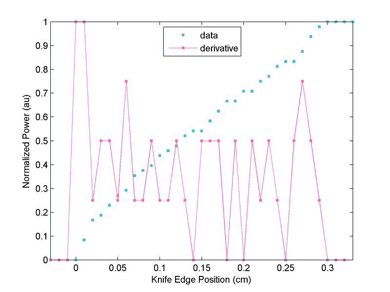
0vtMoLX.png


This doesn't really resemble the actual beam that we have. This is more like what is expected from a rectangular/tophat beam:
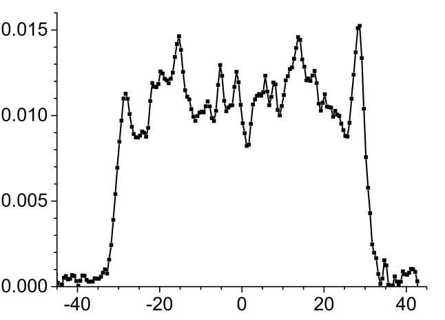
tO4yzyO.jpg


So, what kind of smoothing algorithm can I use on the differentiated data? How do we decide what smoothing would be the most appropriate and accurate in this situation? :confused:

Any help is greatly appreciated.

P. S. I could try to obtain more data points, but I am not sure if that would help. I've used this technique before on Gaussian beams (this time, the raw data was an error function erf) – I had far fewer data points, yet I didn't get this much noise. Why?
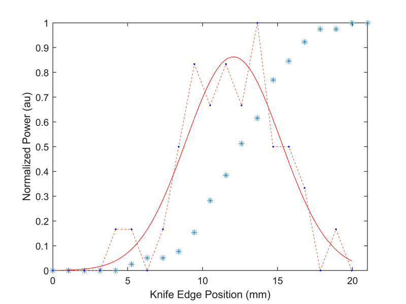
H9wbIb1.png
 

Attachments

  • 0vtMoLX.png
    0vtMoLX.png
    19.4 KB · Views: 1,466
  • tO4yzyO.jpg
    tO4yzyO.jpg
    21.4 KB · Views: 1,291
  • H9wbIb1.png
    H9wbIb1.png
    20.9 KB · Views: 1,136
Mathematics news on Phys.org
  • #2
Your derivative appears to be very discretized: it can assume five different values. The second picture shows a granularity of more than a hundred steps. In the third picture there are only seven different values for the derivaative. Not much either.

Can you increase the intensity, improve the scale on the sensor, or something like that ?
 
  • Like
Likes FactChecker and roam
  • #3
A smaller number of data points means a larger difference between them - noise plays a smaller role. That is something you can do with your data, e.g. combine three adjacent bins to a single bin. Alternatively use one of the many smoothing methods. Just taking a weighted average of bins around your bin should give a nice approximation already.
 
  • Like
Likes roam
  • #4
What you do is fit the original data with something much lower order than the number of data points. Looking at your data, I would recommend a cubic spline with say 5-10 nodes. You then differentiate the low order function analytically.
 
  • Like
Likes roam
  • #5
mfb said:
A smaller number of data points means a larger difference between them - noise plays a smaller role. That is something you can do with your data, e.g. combine three adjacent bins to a single bin. Alternatively use one of the many smoothing methods. Just taking a weighted average of bins around your bin should give a nice approximation already.

Thank you for your suggestions.

So, if I understand correctly, we replace each element with the average of the three adjacent elements. i.e.,

$$\left(y\left(1\right)+y\left(2\right)+y\left(3\right)\right)/3\to y\left(1\right)$$

So we will have ~3x fewer data points to plot. Is that correct?

What if we use Matlab's smooth(.) function with a span 3 moving average filter? This would also be a 3-point smoothing algorithm except we have the same number of data points as we started. Is this method more or less accurate than combining the points?

Here is what I got (smoothed = magenta, original derivative = brown):

Q8q8Zo6.png


I need to reconstruct the actual beam profile as accurately as possible.

BvU said:
Your derivative appears to be very discretized: it can assume five different values. The second picture shows a granularity of more than a hundred steps. In the third picture there are only seven different values for the derivaative. Not much either.

Can you increase the intensity, improve the scale on the sensor, or something like that ?

I can try finding a better power meter. Maybe a digital would be more helpful (this is from an analog output and it is hard to read off minor changes in power).

If I was to use some kind of adjacent average smoothing, would it be helpful to collect more data points?
 

Attachments

  • Q8q8Zo6.png
    Q8q8Zo6.png
    5.8 KB · Views: 1,115
  • #6
More readings for the same curve will probably help.
A slightly more aggressive smoothing should help as well.
 
  • #7
By more aggressive do you mean taking a larger span? I mean, instead of averaging 3 points, you could average a larger number of points.

How would you decide what is a good place to stop smoothing? I've noted that beyond a certain point (in my case, ##\text{span}=33##), you will not see any additional changes to the plot.
 
  • #8
roam said:
By more aggressive do you mean taking a larger span? I mean, instead of averaging 3 points, you could average a larger number of points.
For example, yes. You can also average over points with different weights for them (larger weights for points nearby).

What is best depends on your application.
 
  • Like
Likes roam
  • #9
I would start with a linear regression on the data, then the derivative is just the slope of the line. Check out the r2 value of the regression. Then (looking at the curve) do a third degree regression. Now the derivative is analytically calculable. Again, check the r2 value of this regression. If it is better (higher), stay with the third degree, otherwise use the linear fit.
 
  • Like
Likes suremarc and roam
  • #10
As @BvU pointed out, your data is very crude. I think that you need to address that before post-processing. Smoothing may just be "putting lipstick on a pig." It may mask the information that you are looking for.
 
  • Like
Likes roam
  • #11
Svein said:
I would start with a linear regression on the data, then the derivative is just the slope of the line. Check out the r2 value of the regression. Then (looking at the curve) do a third degree regression. Now the derivative is analytically calculable. Again, check the r2 value of this regression. If it is better (higher), stay with the third degree, otherwise use the linear fit.

So, the idea is to use symbolic differentiation to avoid the noise problem in the numerical computation?

As you suggested, I did fit the data using polynomials of different degree, and here are the first few R2 values:

$$
\begin{array}{c|ccccc}
\hline \text{degree} & 1 & 2 & 3 & 4 & 5\\
\hline R^{2} & 0.9885 & 0.9941 & 0.9945 & 0.9945 & 0.9969
\\\hline \end{array}
$$

I went up to degree 9 and R2 kept increasing. But that might be because we are just modeling the noise in the data at that point.

For the quadratic for instance, you have an equation of the form ##ax^2 + bx + c## which has the analytic derivative ##2ax+b##. But when I plot it, I get this which doesn't look anything like the beam profile:

VWia2od.png

What is wrong here? :confused:

FactChecker said:
As @BvU pointed out, your data is very crude. I think that you need to address that before post-processing. Smoothing may just be "putting lipstick on a pig." It may mask the information that you are looking for.

That is true. But in what way would you say my data is crude?

My data looks like ramp, and this is what I would expect if the beam has a nearly rectangular intensity profile (my signal is its spatial integration). I am not sure in what way I could improve the data except collecting more points...
 

Attachments

  • VWia2od.png
    VWia2od.png
    5.2 KB · Views: 945
  • #12
roam said:
What is wrong here?
Basically nothing. You fit a parabola, you get a parabola. What you want to fit is ideally an almost square block with a lot of detail (*). Try to see what kind of integrated function that would yield.

(*) Detail that is not present in your data: steep edges, with possibly some small deviations on the flat part.
In short: you need higher resolution in both directions: less coarsely rounded off data points an a lot more of them
 
  • Like
Likes roam
  • #13
roam said:
in what way would you say my data is crude?
Sorry, I didn't realize that the derivative was not the raw data. Your calculated derivative numbers have very little resolution -- only 5 descrete values. That is very crude data to work with. In general, taking a derivative, whether symbolically or calculating, will introduce significant noise. Trying to smooth the noise out later is just undoing the derivative, perhaps in a bad way.
 
  • Like
Likes roam
  • #14
The linear regression shows a very high value for r2, so use that for a basic approximation.

Now I (being curious) would subtract the linear regression values from your data and do an FFT on the differences. The lower frequencies of the transformed data might tell you something (try throwing away everything but the three lowest frequencies and transform that back).
 
  • Like
Likes suremarc and roam
  • #15
Hi Svein,

So what is the idea behind subtracting the regression from the data? And are we discarding the high frequencies as being noise?

I did what you suggested. In the DFT, I only kept the 3 lowest terms next to the DC term. Here are the results:

HCPvaxG.png

How can we use this information to reconstruct the beam profile?
 

Attachments

  • HCPvaxG.png
    HCPvaxG.png
    5.2 KB · Views: 874
  • #16
roam said:
How can we use this information to reconstruct the beam profile?
Well, you know much more about the experiment than I do. What I was looking for in the DFT was some regularity in the deviations from the straight line, but there does not seem to be any. My conclusion would be that the linear regression is a very good fit to your experimental data (an r2 of 0.9885 - there are sciences where an r2 of 0.1 is considered exceptionally good) and the deviations are due to noise/measurement accuracy.
 
  • Like
Likes suremarc, roam and FactChecker
  • #17
Svein said:
the deviations are due to noise/measurement accuracy.
I agree. I think that the deltas for the derivatives being such a small set of fixed values shows that the measurement accuracy is a limiting factor and will not allow better results.
 
  • Like
Likes roam
  • #18
FactChecker said:
I agree. I think that the deltas for the derivatives being such a small set of fixed values shows that the measurement accuracy is a limiting factor and will not allow better results.

During my measurements, the increase in data points appeared to occur at fixed increments (that's how I recorded the data). That was the best I could do with my measuring instrument – it wasn't possible to record the values precisely (i.e. using longer decimal format). So, is this what causes the discreteness of the derivative values?

Any explanation would be appreciated.

Svein said:
Well, you know much more about the experiment than I do. What I was looking for in the DFT was some regularity in the deviations from the straight line, but there does not seem to be any. My conclusion would be that the linear regression is a very good fit to your experimental data (an r2 of 0.9885 - there are sciences where an r2 of 0.1 is considered exceptionally good) and the deviations are due to noise/measurement accuracy.

What would the regularities tell us though? As shown in the second figure in my first post, the fluctuations in a tophat beam aren't regular usually...

I guess the only option would be to obtain more precise measurements (more decimal places). I don't see a benefit to using a linear regression in this problem because the analytic derivative would just be a straight line that looks nothing like a beam profile. The analytic differentiation seems to be less useful here than its numerical counterpart.
 
  • #19
roam said:
During my measurements, the increase in data points appeared to occur at fixed increments (that's how I recorded the data). That was the best I could do with my measuring instrument – it wasn't possible to record the values precisely (i.e. using longer decimal format). So, is this what causes the discreteness of the derivative values?
It certainly appears that way.
To keep things simple, suppose one is measuring values between -1.5 and +1.5 but the recorded values are always rounded to the nearest integer -1, 0, +1.
There are only the following 9 cases of (rounded value of ##y_{i+1}##, rounded value of ##y_i##): $$(-1,+1), (-1,0), (-1,-1), (0,+1), (0,0), (0,-1), (+1,+1), (+1,0), (+1,-1).$$ They give the 5 cases for ##y_{i+1} - y_i##: -2, -1, 0, +1, +2.
It appears that these 5 cases correspond to the 5 values that you are getting (except that your Y values trend upward so the deltas are always nonnegative). So it looks like the recorded values are always rounded to values that do not allow very much resolution for the derivative. Any detailed conclusions you reach by analysing the derivative may be saying more about your rounding process than about the derivative itself.
 
Last edited:
  • Like
Likes roam
  • #20
Trying to calculate derivatives on measured data is the equivalent of a high-pass filter: Only the noise gets through.

If you insist on trying to calculate derivatives directly from the data, I'll give you a tip: Instead of doing [itex]f_{n}'=\frac{f_{n+1}-f_{n}}{x_{n+1}-x_{n}} [/itex] (which calculates the secant, not the tangent), try using [itex]f_{n}'=\frac{f_{n+1}-f_{n-1}}{x_{n+1}-x_{n-1}} [/itex] which gives a much better approximation to the tangent.
 
  • Like
Likes DrClaude and roam
  • #21
This is not truly a direct answer but I would recommend something along the lines of reading the eighth chapter in
Davis "Interpolation and approximation ";
https://www.amazon.com/dp/0486624951/?tag=pfamazon01-20
Which is my favorite goto although I am sure that there are probably better books now. The point is that you can choose a sequence of estimators/models, say polynomials of successively higher degrees for instance; take your test models and work from that. The models only have to be linearly independent for this theory to work. Having that in hand you can find the least squares fit/coefficients for the sequence via. a "Gram Matrice" and invert. Once done this model could be reused in similar situations.
Having said that, at the end plot the residuals in "normal probability plot" or nowadays a "Q-Q" plot and see if your residuals fall within the straight line error limits. The "normal probability plot" is my preference since it is really easy to read. Probably you should also try an autocorrelation on the residuals.
Look carefully, if there are systematic variations then you have an opportunity to improve something; i.e. more terms, different modeling sequence.
Improvement beyond a Gaussian (or other physically meaningful error models) is likely worthless. You would be digging in the mud for pearl and would probably find a marble (or worse). Now all of this says you have a simple unencoded type of systems.
You still have to be careful because: if you have Gaussian physical positioning errors and Gaussian electronic/reading noise this will not separate them. There are things you can do; average each individual point by a very slow filter or many readings and averaging. At each point! This is the way to cut down on instrumentation noise. If that's inconvenient rerun your data over and over, and average point by point; this cuts down of instrumentation noise but doesn't reduce instrumentation systematic errors. Truthfully, unless your willing to do this, i.e. reproduce results, you can't expect readers to give reasonable help.
Somewhere I read that Bessel functions (J() ?) can provide a basis for Laser Beam intensity profiles, but I don't remember where and have no experience with these profiles.
 
  • #22
Hi. I'm interested in this problem, so I wanted to ask you a few questions.

I am willing to understand this experiment you are doing. This distribution you are looking for, is the spatial intensity for a laser beam, so when you say this, what you mean is that if for example you are illuminating with this laser to a wall, the shape of the intensity would be something like ##I(x,y)=A e^{-x^2/\sigma^2}e^{-y^2/\sigma^2}##? I don't understand how you would get this from the data you showed.

Do you know of any reference where this experiment is explained? perhaps we can help you if we understand a little bit better what you are doing and the physics behind it.
 
  • #23
So a quadratic fit seems to fit your data quite nicely, therefore the trend through any interval is approximately quadratic. I ask, therefore, what numerical algorithm did you use to calculate the derivatives? The most elementary one, the one I suspect you used, is a forward difference approximation in which the secant between (x,f(x)) to (x+h,f(x+h)) serves as an approximation to the tangent at x. That is, if h is the interval between the abcissae of neighboring points, calculate f(x) and f(x +h) subtract f(x) from f(x+h) and divide by h. Now, let's think geometrically about how well this will fit a curve. If the 'curve' is a straight line, the fit is exact. If the curve has a non-zero second derivative, the FDA is guaranteed to be wrong, how wrong depending on the magnitude of that second derivative.

A central difference approximation requires you evaluate f(x-h) and f(x+h) subtract f(x-h) from f(x+h) and divide by 2h. The intermediate value theorem guarantees that somewhere between x -h and x +h there is a value, c, for which the slope of the secant between (x-h, f(x-h)) and (x+h, f(x+h)) exactly equals the derivative of f(x) at x=c. The CDA doesn't tell us what c is; but at least we know it's somewhere in the symmetric interval around x. In fact, if the curve is a quadratic polynomial, the slope of the CDA secant is the derivative at the midpoint of the interval exactly. Even when the overall f(x) is not quadratic, a quadratic is a good approximation to any well-behaved function anywhere, and the error in the approximation decreases as the interval gets smaller (Think of the first 3 terms of a Taylor series approximation.) To reiterate the clue in the first sentence, your function is approximately quadratic, so the CDA is particularly appropriate. I don't have your data, or I'd try my hand at it. Try it and see if it improves the noise figure of your derivatives.
 
  • Like
Likes Telemachus and roam
  • #24
Hi Svein and Mark Harder, thank you so much for the thorough explanations.

Yes, indeed I had used the forward difference approximation as the simplest approximation for the 1st derivative. In fact, I had generated vectors of differences using diff(.) in Matlab, so that diff(f)./diff(x) would be equivalent to FDA. I will instead try the central difference approximation and see how it goes.

Also: if I obtain high precision data and want to use symbolic computation, would differentiating a quadratic polynomial work? It clearly didn't work using the current data (my post #11)...

@Mark Harder I could send you my data if it helps, but as others suggested I think it is better to obtain more precise data first. I am using high energy lasers so using current modulation I should be able to lower the power and use a very sensitive meter.

@Telemachus Sure thing. Since this thread is under a mathematics forum, I will message you the details of the physics of the setup.
 
  • Like
Likes Telemachus and FactChecker
  • #25
roam said:
would differentiating a quadratic polynomial work?
It would not. Differentiating a quadratic polynomial gives you a straight line. Get it in your head that if you don't see a good profile, all the math in the world won't help you to bring it out from this single very coarse set of data.
 
  • Like
Likes roam
  • #26
roam said:
I think it is better to obtain more precise data first. I am using high energy lasers so using current modulation I should be able to lower the power and use a very sensitive meter.
Good. I agree that getting some data with greater resolution is essential. If you try to use higher order models on data where the largest part is due to round-off, you will get a mess. That being said, the suggestion of using data i-1 and i+1 to estimate i would double the true change of the function value and make the round-off half as significant. (It's also a better way to estimate the slope at point i.) Likewise, using i-2 and i+2 would improve things by a larger factor. But if you carry that to the extreme, you will miss local changes in the function.
 
  • Like
Likes roam
  • #27
roam said:
@Telemachus Sure thing. Since this thread is under a mathematics forum, I will message you the details of the physics of the setup.

Hi again. I already gave a read to your pm. I think the physics is actually important, because it could tell you what function you should be expecting, and what type of function to use for your data. For example, if the data were instead of this intensity profile, just some records for position and time in a free fall at the Earth surface, you would know that it should be a parabola from the physics, and interpolate a parabola, no matter how coarse your data is.

I think that knowing more about the physics in this situation is actually something very important to do the data analysis. Do you have any clue of what type of function you should be expecting?
 
  • Like
Likes roam
  • #28
roam said:
Hi Svein and Mark Harder, thank you so much for the thorough explanations.

Yes, indeed I had used the forward difference approximation as the simplest approximation for the 1st derivative. In fact, I had generated vectors of differences using diff(.) in Matlab, so that diff(f)./diff(x) would be equivalent to FDA. I will instead try the central difference approximation and see how it goes.

Also: if I obtain high precision data and want to use symbolic computation, would differentiating a quadratic polynomial work? It clearly didn't work using the current data (my post #11)...

@Mark Harder I could send you my data if it helps, but as others suggested I think it is better to obtain more precise data first. I am using high energy lasers so using current modulation I should be able to lower the power and use a very sensitive meter.

@Telemachus Sure thing. Since this thread is under a mathematics forum, I will message you the details of the physics of the setup.

Yes, I agree. Having more data and/or better quality data is the best solution if you can do it. You can also increase the also increase the quality of the data by increasing the sampling time for each measurement. The signal/noise ration increases as the square root of the counts (or continuous time). So you'd need to collect four times as long at each point to double the S/N ration. After a while, the time needed becomes impractical; but if you can, spending more time collecting at each point will 'smooth' the data without any risking the distortion of your original data or introducing biases into the experiment.
 
  • Like
Likes roam and FactChecker
  • #29
roam said:
Hi Svein and Mark Harder, thank you so much for the thorough explanations.

Yes, indeed I had used the forward difference approximation as the simplest approximation for the 1st derivative. In fact, I had generated vectors of differences using diff(.) in Matlab, so that diff(f)./diff(x) would be equivalent to FDA. I will instead try the central difference approximation and see how it goes.

Also: if I obtain high precision data and want to use symbolic computation, would differentiating a quadratic polynomial work? It clearly didn't work using the current data (my post #11)...

@Mark Harder I could send you my data if it helps, but as others suggested I think it is better to obtain more precise data first. I am using high energy lasers so using current modulation I should be able to lower the power and use a very sensitive meter.

@Telemachus Sure thing. Since this thread is under a mathematics forum, I will message you the details of the physics of the setup.

Roam, I forgot to mention that I was assuming in my analysis that the x-intervals in your measurements were all equal. If the intervals between points vary across the data, then the problem is more like an interpolation.
 
  • Like
Likes roam

What is smoothing numerical differentiation noise?

Smoothing numerical differentiation noise refers to the process of reducing the noise or fluctuations in a dataset that occurs when performing numerical differentiation. It involves applying a mathematical function or algorithm to the data to remove the noise and create a smoother, more accurate representation of the underlying signal.

Why is it important to smooth numerical differentiation noise?

Smoothing numerical differentiation noise is important because it can improve the accuracy of the data and make it easier to interpret. Noise in a dataset can obscure important patterns or trends, making it difficult to draw meaningful conclusions. By reducing the noise, the data becomes more reliable and useful for analysis.

What are some common techniques for smoothing numerical differentiation noise?

There are several common techniques for smoothing numerical differentiation noise, including moving average, low-pass filters, and Savitzky-Golay filters. These methods involve applying a sliding window or mathematical function to the data to remove the noise and create a smoother result.

How do I choose the best smoothing technique for my data?

The best smoothing technique for your data will depend on the specific characteristics of your dataset and your goals for smoothing. It is important to consider the amount of noise present, the type of noise, and the desired level of smoothing. It may be helpful to experiment with different techniques and compare the results to determine the most effective method for your data.

Are there any potential drawbacks to smoothing numerical differentiation noise?

While smoothing numerical differentiation noise can improve the accuracy and interpretability of data, it can also potentially introduce bias or distort the original signal. It is important to carefully consider the trade-offs and potential limitations of any smoothing technique before applying it to your data.

Similar threads

Replies
11
Views
3K
Replies
8
Views
1K
  • Programming and Computer Science
Replies
6
Views
2K
Replies
6
Views
1K
  • Science and Math Textbooks
Replies
5
Views
2K
  • Programming and Computer Science
Replies
18
Views
2K
Replies
14
Views
2K
  • STEM Academic Advising
Replies
1
Views
1K
  • Computing and Technology
Replies
0
Views
174
Replies
1
Views
791
Back
Top