Math Amateur
Gold Member
MHB
- 3,920
- 48
I am reading Andrew McInerney's book: First Steps in Differential Geometry: Riemannian, Contact, Symplectic ...
I am currently focussed on Chapter 3: Advanced Calculus ... and in particular I am studying Section 3.3 Geometric Sets and Subspaces of [itex]T_p ( \mathbb{R}^n )[/itex] ...
I need help with a basic aspect of Definition 3.3.5 ...
Definition 3.3.5 reads as follows:
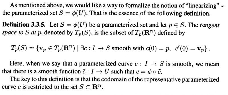 In the above definition we find the following:
" ... ... Here, when we say that a parametrized curve [itex]c \ : \ I \longrightarrow S[/itex] is smooth, we mean that there is a smooth function [itex]\tilde{c} \ : \ I \longrightarrow U[/itex] such that [itex]c = \phi \circ \tilde{c}[/itex] ... ... "
My question is as follows:
Why do we need to bother defining [itex]\tilde{c}[/itex] ... the codomain of [itex]c[/itex] is defined as [itex]S[/itex] ... so we surely only need to stipulate that [itex]c[/itex] is continuously differentiable or [itex]C^1[/itex] ... that is the usual definition of 'smooth' so why isn't this enough ...
... ... so, my question is then, why do we bother defining [itex]\tilde{c}[/itex] and then go on to consider the composite function [itex]c = \phi \circ \tilde{c}[/itex] ... ?Hope someone can help ...
Peter===========================================================
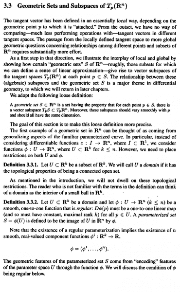
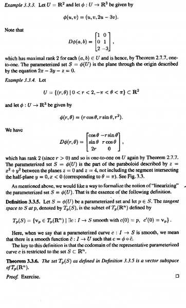
To give the context for McInerney's approach to this definition I am providing the introduction to Section 3.3 as follows:
I am currently focussed on Chapter 3: Advanced Calculus ... and in particular I am studying Section 3.3 Geometric Sets and Subspaces of [itex]T_p ( \mathbb{R}^n )[/itex] ...
I need help with a basic aspect of Definition 3.3.5 ...
Definition 3.3.5 reads as follows:
" ... ... Here, when we say that a parametrized curve [itex]c \ : \ I \longrightarrow S[/itex] is smooth, we mean that there is a smooth function [itex]\tilde{c} \ : \ I \longrightarrow U[/itex] such that [itex]c = \phi \circ \tilde{c}[/itex] ... ... "
My question is as follows:
Why do we need to bother defining [itex]\tilde{c}[/itex] ... the codomain of [itex]c[/itex] is defined as [itex]S[/itex] ... so we surely only need to stipulate that [itex]c[/itex] is continuously differentiable or [itex]C^1[/itex] ... that is the usual definition of 'smooth' so why isn't this enough ...
... ... so, my question is then, why do we bother defining [itex]\tilde{c}[/itex] and then go on to consider the composite function [itex]c = \phi \circ \tilde{c}[/itex] ... ?Hope someone can help ...
Peter===========================================================
To give the context for McInerney's approach to this definition I am providing the introduction to Section 3.3 as follows:
Attachments


