What is the Best Approximation for Heat Transfer in Two-Dimensional Systems?

[c.teixeira]

Hi there.

At first I tought of posting this thread on the homework category, but this is a conceptual doubt rather than anything else.

While revisiting Heat Transfer I stumbled upon a simple problem, that yet got me thinking.

It is as follows:

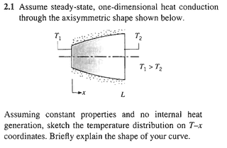
Before anything else, let me show you how they solve the problem:

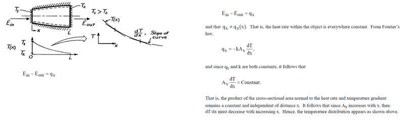
Now, altough I understand and agree with their simple solution, I later tried to apply the heat equation to this problem:

$\frac{\partial(κ\frac{\partial T}{\partial x})}{\partial x}$ + $\frac{\partial(κ\frac{\partialτ}{\partial y})}{\partial y}$ + $\frac{\partial(κ\frac{\partial T}{\partial z})}{\partial z}$ + $\dot{q}$ = $\rho$c$_{p}$$\frac{\partial T}{\partial t}$

Assuming constant properties, no internal heat generation, one-dimensional steady-state heat conduction:

$\frac{\partial(κ\frac{\partial T}{\partial x})}{\partial x}$ = 0 $\Leftrightarrow$ κ$\frac{\partial^{2}T} {\partial x^{2}}$ = 0$\Rightarrow$ T(x) = $C_{1}x$ + $C_{2}$ thus the temperature varies linearly with x.

Comparing this with the solution presented in the image, we see that they are different. Indeed, the solution may take values far apart from the linear solution, depending on the variation of A(x). Rest assured, if A = A(x), then certainly $A_{x}$$\frac{\partial T}{\partial x}$ $\neq$ Constant, as $\frac{\partial T}{\partial x}$ = $C_{1}$.

But the most surprinsing is the following:

If we calculate the expression for the heat transfer rate using the linear solution:

$q_{x}$ = -kA(x)$\frac{\partial T}{\partial x}$ $\Leftrightarrow$ $q_{x}$ = -kA(x)$C_{1}$, and so the heat trasfer rate varies with x through A(x). And this violates the assumption that there is no sink and/or steady state condition.

Now, both the solution presented in the image, and the heat equation ( which I directly applied to this problem) are based on the conservation of energy, so clearly I am missing something. Why are this solutions so unlike if the laws, boundary bonditions and assumptions( namely steady-state, one-dimensional) are the same?

My guess is that this is explained in the following manner:

This two solutions are aproximations to a problem that is not 1 dimensional, but two dimensional. Therefore, they don't need to be equal.

What is your opinion or the matter? If my explanation is suitable, then what is the best approximation and why?


Thank you in advance,

c.teixeira

 

[bigfooted]

The heat equation that you present is for one-dimensional heat conduction with constant cross-sectional area. You have to derive the heat equation for the more general case of non-constant cross-sectional area:

First consider the energy contained in a small volume with area A and thickness $\Delta x$
$E=e A \Delta x$

The change of energy E in time for the volume is 'what comes in minus what comes out'. The 'heat flow' is following Fourier law: $q = -kT_x$

So the balance equation becomes:
$(e(x,t) A(x)\Delta x)_t = q(x,t)A(x) - q(x+\Delta x,t)A(x+\Delta x)$
Now divide by $\Delta x$ and take the limit $\Delta x \rightarrow 0$
$A(x)(e(x,t))_t = -(q(x,t)A(x))_x =-A(x)q_x(x,t) -q(x)A_x(x)$

When $e=\rho cp T$ then,
$A(x)\rho cp T_t = (kT_xA(x))_x = A(x)kT_{xx} + kT_x A_x(x)$

In the steady case you then have:
$A(x)T_{xx} + T_x A_x(x) = 0$
so you are missing a term. Integrating twice leads to
$T(x) = C_2\int\frac{1}{A(x)}dx+ C_1$

 

[c.teixeira]

thank you for your answer bigfooted,

However, I have a hard time agreeing with that explanation.

The heat equation that you present is for one-dimensional heat conduction with constant cross-sectional area. You have to derive the heat equation for the more general case of non-constant cross-sectional area:

$\frac{\partial(κ\frac{\partial T}{\partial x})}{\partial x}$ + $\frac{\partial(κ\frac{\partialτ}{\partial y})}{\partial y}$ + $\frac{\partial(κ\frac{\partial T}{\partial z})}{\partial z}$ + $\dot{q}$ = $\rho$c$_{p}$$\frac{\partial T}{\partial t}$


Correct me if I am wrong (I meant it) but:

The heat equation I presented, re-posted above, is the most general form of the heat diffusion equation in Cartesian coordinates. It holds, regardless of the geometry of the problem. For example, one could apply the heat equation I presented to the study of heat on a sphere, altough that would be both laborious and unnecessary since spherical coordinates would be more suitable.

As to the rest of the derivation you presented, I agree with it. It seems right to me. But it is just the "formal" derivation of the solution "they" used to solve the problem. And that is indeed the issue. Why are this solutions so different, if they are both correct?

So, if I am right about my first paragraph, the question remains. More specificly:

]My guess is that this is explained in the following manner:

This two solutions are aproximations to a problem that is not 1 dimensional, but two dimensional. Therefore, they don't need to be equal.

What is your opinion or the matter? If my explanation is suitable, then what is the best approximation and why?

Any opinions on the matter are welcome,

c.teixeira

 

[256bits]

But the most surprinsing is the following:

If we calculate the expression for the heat transfer rate using the linear solution:

q_{x}qx = -kA(x)\frac{\partial T}{\partial x}Tx \Leftrightarrow q_{x}qx = -kA(x)C_{1}C1, and so the heat trasfer rate varies with x through A(x). And this violates the assumption that there is no sink and/or steady state condition.

Now, both the solution presented in the image, and the heat equation ( which I directly applied to this problem) are based on the conservation of energy, so clearly I am missing something. Why are this solutions so unlike if the laws, boundary bonditions and assumptions( namely steady-state, one-dimensional) are the same?

They stopped before evaluating the one-dimensional equation, saying that Ax( dT/dx ) must be constant, knowing that the area changes.
You evaluated the equation as simply one dimensional heat flow with no area change.

The problem is an execution of how flows other than one dimensional, can be analyzed and solved by using the simpler one dimensional Fourier law, with correct assumptions, rather than using the all inclusive three dimensional equation.

 

[c.teixeira]

The problem is an execution of how flows other than one dimensional, can be analyzed and solved by using the simpler one dimensional Fourier law, with correct assumptions, rather than using the all inclusive three dimensional equation.

Ok, I undestood your explanation. It makes sense. It is much like the explanation I tough to myself.


Thank you,