- #1
Math Amateur
Gold Member
MHB
- 3,990
- 48
I am reading Andrew Browder's book: "Mathematical Analysis: An Introduction" ... ...
I am currently reading Chapter 8: Differentiable Maps and am specifically focused on Section 8.2 Differentials ... ...
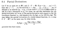
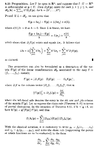
I need some help with fully understanding some remarks by Browder made after the proof of Proposition 8.21 ... ...Proposition 8.21 (including some preliminary material and some remarks after the proof) reads as follows:View attachment 9443
View attachment 9444
After the proof of Proposition 8.21, Browder makes the following remarks:
" ... ... This proposition can also be formulated as a description of the matrix \(\displaystyle f'(p)\) of the linear transformation \(\displaystyle \text{df}_p\) associated with the map \(\displaystyle f = ( f_1, \ldots , f_m )\) namely
\(\displaystyle f'(p) = [ \ D_1 f(p) \ \ D_2 f(p) \ \ldots \ D_n f(p)]\)
where \(\displaystyle D_jf\) is the column vector \(\displaystyle [D_jf_1, \ldots , D_jf_m ]^t\), that is \(\displaystyle ( f'(p) )_j^i = D_jf_i(p) = \frac{ \partial f_i }{ \partial x_j }\) where the left-hand side denotes the entry in the ith row and jth column of the matrix \(\displaystyle f'(p)\) ...
... ... ... "
My questions are as follows ...How/why exactly do we know that
\(\displaystyle f'(p) = [ \ D_1 f(p) \ \ D_2 f(p) \ \ldots \ D_n f(p)]\) ... ... and further ...How/why exactly do we know that
\(\displaystyle ( f'(p) )_j^i = D_jf_i(p) = \frac{ \partial f_i }{ \partial x_j }\) ...
Help will be much appreciated ...
Peter
I am currently reading Chapter 8: Differentiable Maps and am specifically focused on Section 8.2 Differentials ... ...
I need some help with fully understanding some remarks by Browder made after the proof of Proposition 8.21 ... ...Proposition 8.21 (including some preliminary material and some remarks after the proof) reads as follows:View attachment 9443
View attachment 9444
After the proof of Proposition 8.21, Browder makes the following remarks:
" ... ... This proposition can also be formulated as a description of the matrix \(\displaystyle f'(p)\) of the linear transformation \(\displaystyle \text{df}_p\) associated with the map \(\displaystyle f = ( f_1, \ldots , f_m )\) namely
\(\displaystyle f'(p) = [ \ D_1 f(p) \ \ D_2 f(p) \ \ldots \ D_n f(p)]\)
where \(\displaystyle D_jf\) is the column vector \(\displaystyle [D_jf_1, \ldots , D_jf_m ]^t\), that is \(\displaystyle ( f'(p) )_j^i = D_jf_i(p) = \frac{ \partial f_i }{ \partial x_j }\) where the left-hand side denotes the entry in the ith row and jth column of the matrix \(\displaystyle f'(p)\) ...
... ... ... "
My questions are as follows ...How/why exactly do we know that
\(\displaystyle f'(p) = [ \ D_1 f(p) \ \ D_2 f(p) \ \ldots \ D_n f(p)]\) ... ... and further ...How/why exactly do we know that
\(\displaystyle ( f'(p) )_j^i = D_jf_i(p) = \frac{ \partial f_i }{ \partial x_j }\) ...
Help will be much appreciated ...
Peter