Geodesic path in 2 dimensions?

[James1238765]

TL;DR Summary

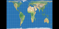
What is the correct Christoffel numerical values for every point $[x,y]$ mapping a spherical surface to a plane surface?

The object takes a step [x, y] in 2 dimensional space. This is represented the change in coordinate $x \vec e_x + y \vec e_y$ where $e_x$ and $e_y$ are basis vectors in this space.

Suppose we define a non-linear / parametric transformation of this $\vec e_x$ and $\vec e_y$ basis vectors using 4 numbers defined all throughout the grid, specifying how each basis vector should transform into a second space.

1. When the transform maps $e_x \rightarrow e_{xprime}$ and $e_y \rightarrow e_{yprime}$, we get equivalent traced paths over time.

2. When the transform adds random noise between the basis vectors, we get:

What is the correct parametric specification of the individual numbers $R_x^x, R_y^x, R_x^y, R_y^y$ on this grid of four reals numbers $[R_x^x, R_y^x, R_x^y, R_y^y]$ defined explicitly on every grid point $[x,y]$, that will trace the correct great circle path of a plane flying straight through the earth (geodesic line on a spherical surface)?

 

[pasmith]

It depends on the particular projection in use.

Parametrize the sphere as $$\begin{split} X &= \cos \lambda \cos \theta \\ Y &= \sin \lambda \cos \theta \\ Z &= \sin \theta \end{split}$$ for longitude $\lambda$ and latitude $\theta$. Then the distance element is $$ds^2 = dX^2 + dY^2 + dZ^2 = \cos^2(\theta)\,d\lambda^2 + d\theta^2.$$ The projection is usually defined as a function $(\lambda, \theta) \mapsto (x,y)$, but really you want to do the reverse so that $$\begin{split} ds^2 &= \cos^2(\theta)\,d\lambda^2 + d\theta^2 \\ &= (\lambda_x^2 \cos^2(\theta) + \theta_x^2)\,dx^2 + 2(\lambda_x \lambda_y \cos^2(\theta) + \theta_x\theta_y)\,dx\,dy + (\lambda_y^2 \cos^2(\theta) + \theta_y^2)\,dy^2\end{split}$$ where the subscripts denote partial derivatives. From this metric you can calculate the Christoffel symbols of a particular projection. For the Mercator projection, $$x = \lambda, \qquad y = \ln(\sec \theta + \tan \theta)$$ we have $$\lambda = x, \qquad \theta = \arctan(\sinh y).$$

 

[James1238765]

@pasmith thank you. I did some exploration on the mercartor transformation.

As the earth is a sphere of roughly constant radius R, 2 coordinates $[longitude, latitude]$ are sufficient to describe the location of any point on earth uniquely. We exclude singular points at the north and south pole. By convention we define the [0,0] coordinate to be that of Null Island:

We might construct a "equal projection map" of this sphere onto a 2D plane, by chopping the 360 slices of longitude into equal x slices, and the 178 (-89 to + 89) slices of latitude into equal y slices as follows:

( from [here]. Note the equal rectangular spacing of the grid.)

Next, we define the Mercartor transformation according to [here]. Massaging the coordinates so that [0,0] is the top left of the image, we can obtain the direct 1-to-1transformation on the x axis, and a stretched transformation on the y axis (for each $x_0$ held in place). We obtain the computed Mercartor transformation:

(Note the resulting uneven spacing of the previously equal sized grid.) From visual inspection, this agrees with commonly seen Mercartor projection of the earth, for example [here]:

 

[James1238765]

The Christoffel coefficients are scalar real numbers that encode the change of each basis vectors, in terms of those same basis vectors themselves, at every point.

1. Polar transformation

We define a transformation between coordinates $\{x, y\} \rightarrow \{a,b\}$ as follows:

$$ x := a \cos b $$
$$y := a \sin b $$

Thus any vector $\vec r$ in xy coordinates can be represented also as

$$\vec r = \begin{pmatrix} a \cos b \\ a \sin b \end{pmatrix}$$

in terms of ab coordinates.

We define basis vectors $\vec E_a, \vec E_b$ as follows:

$$ \vec E_a = \frac{d \vec r}{da} = \begin{pmatrix} \cos b \\ \sin b \end{pmatrix} $$

$$ \vec E_b = \frac{d \vec r}{db} = \begin{pmatrix} -a \sin b \\ a \cos b \end{pmatrix} $$

and coefficients set $C_{ij}$ as follows:

$$ C_{ij} = \frac{d \vec i}{dj} = \Gamma_{ij}^a \vec E_a + \Gamma_{ij}^b \vec E_b$$

Permuting over all possible combinations of i and j, we obtain

$$ C_{aa} = \frac{d \vec E_a}{da} = \begin{pmatrix} 0 \\ 0 \end{pmatrix} = 0 \vec E_a + 0 \vec E_b $$

$$C_{ab} = \frac{d \vec E_a}{db} = \begin{pmatrix} - \sin b \\ \cos b \end{pmatrix} = 0 \vec E_a + \frac{1}{a} \vec E_b $$

$$C_{ba} = \frac{d \vec E_b}{da} = \begin{pmatrix} - \sin b \\ \cos b \end{pmatrix} = 0 \vec E_a + 0 \vec E_b $$

$$C_{bb} = \frac{d \vec E_b}{db} = \begin{pmatrix} -a \cos b \\ -a \sin b \end{pmatrix} = -1 \vec E_a + 0 \vec E_b $$

------------------------------------------------

2. Spherical polar transformation

We define a transformation between coordinates $\{x, y,z\} \rightarrow \{a,b,c\}$ as follows:

$$ x := a \sin b \cos c$$
$$ y := a \sin b \sin c$$
$$ z := a \cos b$$

Thus any vector $\vec r$ in xyz coordinates can be represented also as

$$\vec r = \begin{pmatrix} a \sin b \cos c \\ a \sin b \sin c \\ a \cos b \end{pmatrix}$$

in terms of abc coordinates.

We define basis vectors $\vec E_a, \vec E_b, \vec E_c$ as follows:

$$ \vec E_a = \frac{d \vec r}{da} = \begin{pmatrix} \sin b \cos c \\ \sin b \sin c \\ \cos b \end{pmatrix} $$

$$ \vec E_b = \frac{d \vec r}{db} = \begin{pmatrix} a \cos b \cos c \\ a \cos b \sin c \\ -a \sin b \end{pmatrix} $$

$$ \vec E_c = \frac{d \vec r}{dc} = \begin{pmatrix} -a \sin b \sin c \\ a \sin b \cos c \\ 0 \end{pmatrix} $$

and coefficients set $C_{ij}$ as follows:

$$ C_{ij} = \frac{d \vec i}{dj} = \Gamma_{ij}^a \vec E_a + \Gamma_{ij}^b \vec E_b + \Gamma_{ij}^c \vec E_c $$

Permuting over all possible combinations of i and j, we obtain

$$C_{aa} = \frac{d \vec E_a}{da} = \begin{pmatrix} 0 \\ 0 \\ 0 \end{pmatrix} = 0 \vec E_a + 0 \vec E_b + 0 \vec E_c$$

$$C_{ab} = \frac{d \vec E_a}{db} = \begin{pmatrix} \cos b \cos c \\ \cos b \sin c \\ -\sin b \end{pmatrix} = 0 \vec E_a + \frac{1}{a} \vec E_b + 0 \vec E_c$$

$$C_{ac} = \frac{d \vec E_a}{dc} = \begin{pmatrix} -\sin b \sin c \\ \sin b \cos c \\ 0 \end{pmatrix} = 0 \vec E_a + 0 \vec E_b + \frac{1}{a} \vec E_c$$

$$C_{ba} = \frac{d \vec E_b}{da} = \begin{pmatrix} \cos b \cos c \\ \cos b \sin c \\ -\sin b \end{pmatrix} = 0 \vec E_a +\frac{1}{a} \vec E_b + 0 \vec E_c$$

$$C_{bb} = \frac{d \vec E_b}{db} = \begin{pmatrix} -a \sin b \cos c \\ -a \sin b \sin c \\ -a \cos b \end{pmatrix} = -a \vec E_a + 0 \vec E_b + 0 \vec E_c$$

$$C_{bc} = \frac{d \vec E_b}{dc} = \begin{pmatrix} -a \cos b \sin c \\ a \cos b \cos c \\ 0 \end{pmatrix} = 0 \vec E_a + 0 \vec E_b + \frac{cos b}{sin b} \vec E_c$$

$$C_{ca} = \frac{d \vec E_c}{da} = \begin{pmatrix} - \sin b \sin c \\ \sin b \cos c \\ 0 \end{pmatrix} = 0 \vec E_a + 0 \vec E_b + \frac{1}{a} \vec E_c$$

$$C_{cb} = \frac{d \vec E_c}{db} = \begin{pmatrix} -a \cos b \sin c \\ a \cos b \cos c \\ 0 \end{pmatrix} = 0 \vec E_a + 0 \vec E_b - \frac{\cos b}{\sin b} \vec E_c$$

$$C_{cc} = \frac{d \vec E_c}{dc} = \begin{pmatrix} - a \sin b \cos c \\ - a \sin b \sin c \\ 0 \end{pmatrix} ?= -a \sin^2 b \vec E_a + -\sin b \cos b \vec E_b + 0 \vec E_c$$

$C_{cc}$ is the first non-trivial complicated linear combinations of $\vec E_a, \vec E_b, \vec E_c$ encountered so far. I am unclear about how trigonometric identitites can equate the left hand side and right hand side. Following [this] at (10:00):

I am unable to follow how the $3^{rd}$ equal signs can simplify overall to the $4^{th}$ equal sign in the above calculation?

 

[James1238765]

Alternative calculation using $g$ (metric) algebra:

1. Polar coordinates

Starting from the definition of $E_a$ and $E_b$:

$$ E_a = \begin{pmatrix} \cos b \\ \sin b \end{pmatrix} $$
$$E_b = \begin{pmatrix} -a \sin b \\ a \cos b \end{pmatrix}$$

we further define $g_{ij}$ to be:

$$ g_{ij} = \begin{bmatrix} E_a \cdot E_a \ E_a \cdot E_b \\ E_b \cdot E_a \ E_b \cdot E_b \end{bmatrix} = \begin{bmatrix} 1 \ 0 \\ 0 \ a^2 \end{bmatrix}$$

and $g^{ij}$ calculated termwise from $g_{ij}$ as follows:

$$ g_{aa}g^{aa} + g_{ab}g^{ba} = 1$$
$$ g_{aa}g^{ab} + g_{ab}g^{bb} = 0$$
$$ g_{ba}g^{aa} + g_{bb}g^{ba} = 0$$
$$ g_{ba}g^{ab} + g_{bb}g^{bb} = 1$$

Calculating over each known $g_{ij}$, we obtain

$$ g^{ij} = \begin{bmatrix} 1 \ 0 \\ 0 \ \frac{1}{a^2} \end{bmatrix}$$

The Christoffel coefficients can be calculated according to the formula:

$$ \Gamma^i_{jk} = \frac{1}{2} g^{i\Sigma} \begin{pmatrix} \frac{dg_{i\Sigma}}{dk} + \frac{dg_{k\Sigma}}{dj} - \frac{dg_{jk}}{d\Sigma} \end{pmatrix}$$

where $\Sigma$ is summed over all coordinates $\{a, b\}$, ie:

$$ \Gamma^i_{jk} = \frac{1}{2}g^{ia} \begin{pmatrix} \frac{dg_{ia}}{dk} + \frac{dg_{ka}}{dj} - \frac{dg_{jk}}{da} \end{pmatrix} + \frac{1}{2}g^{ib} \begin{pmatrix} \frac{dg_{ib}}{dk} + \frac{dg_{kb}}{dj} - \frac{dg_{jk}}{db} \end{pmatrix}$$

Therefore,

$$ \Gamma^a_{aa} = \frac{1}{2}g^{aa} \begin{pmatrix} \frac{dg_{aa}}{da} + \frac{dg_{aa}}{da} - \frac{dg_{aa}}{da} \end{pmatrix} + \frac{1}{2}g^{ab} \begin{pmatrix} \frac{dg_{ab}}{da} + \frac{dg_{ab}}{da} - \frac{dg_{aa}}{db} \end{pmatrix} = \frac{1}{2}(1)(0) = 0$$

$$ \Gamma^b_{aa} = \frac{1}{2}g^{ba} \begin{pmatrix} \frac{dg_{ba}}{da} + \frac{dg_{aa}}{da} - \frac{dg_{aa}}{da} \end{pmatrix} + \frac{1}{2}g^{bb} \begin{pmatrix} \frac{dg_{bb}}{da} + \frac{dg_{ab}}{da} - \frac{dg_{aa}}{db} \end{pmatrix} = \frac{1}{2}(\frac{1}{a^2})(2a) = \frac{1}{a}$$

$$ \Gamma^a_{ab} = \frac{1}{2}g^{aa} \begin{pmatrix} \frac{dg_{aa}}{db} + \frac{dg_{ba}}{da} - \frac{dg_{ab}}{da} \end{pmatrix} + \frac{1}{2}g^{ab} \begin{pmatrix} \frac{dg_{ab}}{db} + \frac{dg_{bb}}{da} - \frac{dg_{ab}}{db} \end{pmatrix} = \frac{1}{2}(1)(0) = 0$$

$$ \Gamma^b_{ab} = \frac{1}{2}g^{ba} \begin{pmatrix} \frac{dg_{ba}}{db} + \frac{dg_{ba}}{da} - \frac{dg_{ab}}{da} \end{pmatrix} + \frac{1}{2}g^{bb} \begin{pmatrix} \frac{dg_{bb}}{db} + \frac{dg_{bb}}{da} - \frac{dg_{ab}}{db} \end{pmatrix} = \frac{1}{2}(\frac{1}{a^2})(0) = 0$$

$$ \Gamma^a_{ba} = \frac{1}{2}g^{aa} \begin{pmatrix} \frac{dg_{aa}}{da} + \frac{dg_{aa}}{db} - \frac{dg_{ba}}{da} \end{pmatrix} + \frac{1}{2}g^{ab} \begin{pmatrix} \frac{dg_{ab}}{da} + \frac{dg_{ab}}{db} - \frac{dg_{ba}}{db} \end{pmatrix} = \frac{1}{2}(1)(0) = 0$$

$$ \Gamma^b_{ba} = \frac{1}{2}g^{ba} \begin{pmatrix} \frac{dg_{ba}}{da} + \frac{dg_{aa}}{db} - \frac{dg_{ba}}{da} \end{pmatrix} + \frac{1}{2}g^{bb} \begin{pmatrix} \frac{dg_{bb}}{da} + \frac{dg_{ab}}{db} - \frac{dg_{ba}}{db} \end{pmatrix} = \frac{1}{2}(\frac{1}{a^2}_(2a) = \frac{1}{a}$$

$$ \Gamma^a_{bb} = \frac{1}{2}g^{aa} \begin{pmatrix} \frac{dg_{aa}}{db} + \frac{dg_{ba}}{db} - \frac{dg_{bb}}{da} \end{pmatrix} + \frac{1}{2}g^{ib} \begin{pmatrix} \frac{dg_{ab}}{db} + \frac{dg_{bb}}{db} - \frac{dg_{bb}}{db} \end{pmatrix} = \frac{1}{2}(10)(-2a) = -a $$

$$ \Gamma^b_{bb} = \frac{1}{2}g^{ba} \begin{pmatrix} \frac{dg_{ba}}{db} + \frac{dg_{ba}}{db} - \frac{dg_{bb}}{da} \end{pmatrix} + \frac{1}{2}g^{bb} \begin{pmatrix} \frac{dg_{bb}}{db} + \frac{dg_{bb}}{db} - \frac{dg_{bb}}{db} \end{pmatrix} = \frac{1}{2}(\frac{1}{a^2})(0) = 0$$

---------------------------------------------

In summary, the complete calculated values are:

$$ \Gamma^a_{aa} = 0, \Gamma^b_{aa} = \frac{1}{a}, \Gamma^a_{ab} = 0, \Gamma^b_{aa} = \frac{1}{a}$$
$$ \Gamma^a_{ba} = 0, \Gamma^b_{ba} = \frac{1}{a}, \Gamma^a_{bb} = -a, \Gamma^b_{bb} = 0$$

which agrees with the calculation using the first method above, *except* for $\Gamma^b_{aa}$ which yielded 0 by the first method, but $\frac{1}{a}$ by the second method (?)

 

[James1238765]

The geodesic path around the surface of the earth can be deduced as follows:

A geodesic path $s$ on the 2 dimensional coordinate space $\{a,b\}$ is defined to be any path on $\{a,b\}$ space that satisfies both the set of 2 equations

$$ \frac{da}{ds^2} + \Gamma^a_{aa} \frac{da}{ds} \frac{da}{ds} + \Gamma^a_{ab} \frac{da}{ds} \frac{db}{ds} + \Gamma^a_{ba} \frac{db}{ds} \frac{da}{ds} + \Gamma^a_{bb} \frac{db}{ds} \frac{db}{ds} = 0$$

$$ \frac{db}{ds^2} + \Gamma^b_{aa} \frac{da}{ds} \frac{da}{ds} + \Gamma^b_{ab} \frac{da}{ds} \frac{db}{ds} + \Gamma^b_{ba} \frac{db}{ds} \frac{da}{ds} + \Gamma^b_{bb} \frac{db}{ds} \frac{db}{ds} = 0$$

For the case of the earth surface, where the longitude and latitude coordinates $\{a,b\}$ are mapped onto three dimensional $\{x,y,z\}$ coordinates as follows (latitude is defined as 0 at the north pole, 180 degrees at the south pole):

$$ \vec r = \begin{pmatrix} \cos b \sin a \\ \sin b \sin a \\ \cos a \end{pmatrix} $$

It can be calculated that the 8 Christoffel coefficients will be:

$$ \Gamma^a_{aa} = 0 , \Gamma^b_{aa} = 0 , \Gamma^a_{ab} = 0 , \Gamma^b_{ab} = \frac{\cos a}{\sin a}$$
$$ \Gamma^a_{ba} = 0 , \Gamma^b_{ba} = \frac{\cos a}{\sin a} , \Gamma^a_{bb} = -\cos a \sin a , \Gamma^b_{ab} = 0$$

which reduces the geodesic path conditions to:

$$ \frac{da}{ds^2} - \cos a \sin a \frac{db}{ds} \frac{db}{ds} = 0$$

$$ \frac{db}{ds^2} + \frac{\cos a}{\sin a} \frac{da}{ds} \frac{db}{ds} +\frac{\cos a}{\sin a} \frac{db}{ds} \frac{da}{ds} = 0$$

From here, it may be possible to guess a parametrization for $s$ which will force both equations to be identically $0$.

Following [this] we guess the following parametrization $s$:

$$ a = a_0 , b = s$$

for some fixed constant latitude $a_0$, and traveling along the longitude $b$ in the manner of $s$. Then,

$$ \frac{da}{ds} = 0 , \frac{d^2a}{ds^2} = 0$$
$$ \frac{db}{ds} = 1 , \frac{d^2b}{ds^2} = 0$$

Substituting into the geodesic path conditions, we get:

$$ - \cos a_0 \sin a_0 = 0 $$
$$ 0 = 0 $$

The second equation is identically zero. The first equation can be $0$ if either $\sin a_0 = 0$, which correspond to the singular point path at the north pole or south pole, or $\cos a_0 = 0$, which corresponds to a path along the equator.

By spherical symmetry, all paths along the "widest diameter of the earth" is therefore also a geodesic path. A geodesic path on the earth surface is a plane the cuts through the center of the earth sphere connecting the two locations.

 

[James1238765]

1. In the case of 2D plane $\{a,b\}$ embedded onto a 3D surface $\{x,y,z\}$ in the manner of above:

$$ \vec r = \begin{pmatrix} \cos b \sin a \\ \sin b \sin a \\ \cos a \end{pmatrix} $$

The numerical values of the various Christoffel coefficients are checked to be in the range:

which agrees with analytically parametrized values for $\Gamma$ above. The zero values satisfying all the geodesic conditions are found only on the line going through the equator:

2. We extend the dimension by one, into the case of a 3D volume $\{a,b,c\}$ being embedded onto a 4D surface $\{w,x,y,z\}$ in the manner of:

$$ \vec r = \begin{pmatrix} \cos a \\ \sin a \cos b \\ \sin a \sin b \cos b \\ \sin a \sin b \sin c \end{pmatrix} $$

The numerical range of the Christoffel coefficients are:

 

[James1238765]

1. Removing the terms of $\Gamma$ which are identically zero, the geodesic conditions reduce to the set of 3 equations:

$$ \frac{d^2a}{ds^2} + \Gamma^a_{bb}\frac{db}{ds}\frac{db}{ds} + \Gamma^a_{cc}\frac{dc}{ds}\frac{dc}{ds} = 0$$

$$ \frac{d^2b}{ds^2} + \Gamma^b_{aa}\frac{da}{ds}\frac{da}{ds} + \Gamma^b_{ab}\frac{da}{ds}\frac{db}{ds} + \Gamma^b_{ba}\frac{db}{ds}\frac{da}{ds} + \Gamma^b_{ca}\frac{dc}{ds}\frac{da}{ds} + \Gamma^b_{cc}\frac{dc}{ds}\frac{dc}{ds}= 0$$

$$ \frac{d^2c}{ds^2} + \Gamma^c_{aa}\frac{da}{ds}\frac{da}{ds} + \Gamma^a_{av}\frac{da}{ds}\frac{db}{ds} + \Gamma^c_{ac}\frac{da}{ds}\frac{dc}{ds} + \Gamma^c_{bb}\frac{db}{ds}\frac{db}{ds} + \Gamma^c_{bc}\frac{db}{ds}\frac{dc}{ds} $$
$$+ \Gamma^c_{ca}\frac{dc}{ds}\frac{da}{ds} + \Gamma^c_{cb}\frac{dc}{ds}\frac{db}{ds}= 0$$

Following similar reasoning as in the lower dimension, there must be a geodesic path traveling along one axis (while keeping the other 2 axes constant), so that this path can be rotated into any other geodesic path on the hypersphere.

Testing $a = s, b = b_0, c = c_0$ does not give any path where the geodesic equations are zero everywhere.

Testing $a = a_0, b = s, c = c_0$ also does not give any path where the geodesic equations are zero everywhere.

Testing $a = a_0, b = b_0, c = s$ yields the numerical solution by setting $a = \frac{\pi}{2}$ and $b = \frac{\pi}{2}$, ie. into the midpoint of the ab plane. The 3 geodesic conditions equals 0 for all s, using these setting.

By symmetry argument, all higher dimensional spheres should also have a geodesic line at the midpoint at all the other coordinates, while travelling along the line of a special axis.

----------------------------------------------

2. The Riemann curvature tensor can be calculated once the Christoffel coefficients $\Gamma$ are known everywhere, according to the formula:

$$ R^i_{jkl} = \frac{d\Gamma^i_{jl}}{dk} - \frac{d\Gamma^i_{jk}}{dl} + \Gamma^i_{\Sigma k} \Gamma^\Sigma _{jl} - \Gamma^i _{\Sigma l} \Gamma^\Sigma _{jk}$$

3. The Ricci curvature is a trace-like summary of the Riemann curvature according to the formula:

$$ R_{ij} = R^a_{iaj} + R^b_{ibj} + R^c_{icj}$$

4. The Ricci scalar can be calculated using the Ricci curvature and the $g^{ij}$ values at each point:

$$ R = g^{aa}R_{aa} + g^{ab}R_{ab} + g^{ac}R_{ac} + g^{ba}R_{ba} + g^{bb}R_{bb} + g^{bc}R_{bc} + g^{ca}R_{ca} + g^{cb}R_{cb} + g^{cc}R_{cc}$$

5. The left hand side of the general relativity field equation requires one more constant $\Lambda =2.036 \times 10^{-35}$ and is calculated at each point according to the expression:

$$ R_{ij} + R g^{ij} + \Lambda g^{ij} $$

 

[pbuk]

What are you actually trying to do?

A geodesic path on the earth surface is a plane the cuts through the center of the earth sphere connecting the two locations.

I think you mean a geodesic path on the Earth's surface (modelled as a perfect sphere) lies in a plane containing the center of the sphere and the two locations.

This is known as a great circle path, and the fact that it is a geodesic (i.e. the shortest distance between two points) is well known and more easily proven.

https://mathworld.wolfram.com/SphericalGeometry.html

 

[James1238765]

1. In the case of the 4D volume $\{a,b,c,d\}$ described via the $g_{ij}$ Schwartzchild-like matrix:

$$ g_{ij} = \begin{pmatrix} \frac{1}{b} -1 & 0 & 0 & 0 \\ 0 & \frac{1}{1 - \frac{1}{b}} & 0 & 0 \\ 0 & 0 & b^2 & 0 \\ 0 & 0 & 0 & b^2 \sin^2 c \end{pmatrix} $$

The numerical $4 \times 4 \times 4 = 64$ Christoffel coefficients are in the range:

The numerical $4 \times 4 \times 4 \times 4 = = 256$ Riemann curvature are not identically zero:

However, the $4 \times 4 = 16$ Ricci curvature are zero:

The 1 Ricci scalar is also (likely) zero:

-----------------------------------------------

2. In the case of the 4D volume $\{a,b,c,d\}$ described via the $g_{ij}$ Kerr-like matrix:

$$ g_{ij} = \begin{pmatrix} -b & 0 & 0 & b \sin^2 c \\ 0 & \frac{1}{b^2} & 0 & 0 \\ 0 & 0 & 1 & 0 \\ b \sin^2 c & 0 & 0 & b \sin^2 c (b + \sin^2 c) \end{pmatrix} $$

 

[Mark44]

@James1238765, most of the images in your previous post, #10, are unreadable due to their small size. For this reason, whatever it is that you're doing is of use only to yourself.

Also, in the LaTeX for matrices, use & to separate individual elements of a row, not \. To separate rows, use \\, which you did. I have edited the two matrices in post #10.

 

[James1238765]

The 4 geodesic conditions in 4 dimensions are:

$$\frac{d^2\Lambda}{ds^2} + \Gamma^\Lambda_{aa}\frac{da}{ds}\frac{da}{ds} + \Gamma^\Lambda_{ab}\frac{da}{ds}\frac{db}{ds} + \Gamma^\Lambda_{ac}\frac{da}{ds}\frac{dc}{ds} +\Gamma^\Lambda_{ad}\frac{da}{ds}\frac{dd}{ds}+\Gamma^\Lambda_{ba}\frac{db}{ds}\frac{da}{ds}+\Gamma^\Lambda_{bb}\frac{db}{ds}\frac{db}{ds}$$
$$+\Gamma^\Lambda_{bc}\frac{db}{ds}\frac{dc}{ds}+\Gamma^\Lambda_{bd}\frac{db}{ds}\frac{dd}{ds}+\Gamma^\Lambda_{ca}\frac{dc}{ds}\frac{da}{ds}+\Gamma^\Lambda_{cb}\frac{dc}{ds}\frac{db}{ds}+\Gamma^\Lambda_{cc}\frac{dc}{ds}\frac{dc}{ds}+\Gamma^\Lambda_{cd}\frac{dc}{ds}\frac{dd}{ds}+\Gamma^\Lambda_{da}\frac{dd}{ds}\frac{da}{ds}$$
$$+\Gamma^\Lambda_{db}\frac{dd}{ds}\frac{db}{ds}+\Gamma^\Lambda_{dc}\frac{dd}{ds}\frac{dc}{ds}+\Gamma^\Lambda_{dd}\frac{dd}{ds}\frac{dd}{ds} = 0$$

for each $\Lambda = \{a, b, c, d\}$.

1. In the case of Schwarchild metric, there are 13 (out of 64) non-zero Christoffel coefficients:

$$\Gamma^r_{tt} = \frac{M(r - 2M)}{r^3}$$
$$\Gamma^r_{rr} = \frac{M}{r(r - 2M)}$$
$$\Gamma^r_{\theta \theta} = -(r-2M)$$
$$\Gamma^r_{\phi \phi} = -(r-2M) \sin^2 \theta$$
$$\Gamma^t_{rt} = \frac{M}{r(r-2M)}$$
$$\Gamma^t_{tr} = \frac{M}{r(r-2M)}$$
$$\Gamma^\theta_{r \theta} = \frac{1}{r}$$
$$\Gamma^\theta_{\theta r} = \frac{1}{r}$$
$$\Gamma^\theta-{\phi \phi} = -\sin \theta \cos \theta$$
$$\Gamma^\phi_{r \phi} = \frac{1}{r}$$
$$\Gamma^\phi_{\phi r} = \frac{1}{r}$$
$$\Gamma^\phi_{\theta \phi} = \frac {\cos \theta}{\sin \theta}$$
$$\Gamma^\phi_{\phi \theta} = \frac {\cos \theta}{\sin \theta}$$

Removing the Christoffel coefficients that are identically zero, the geodesic conditions reduce to the set of 4 equations:

$$\frac{d^2t}{ds^2} + 2\frac{M}{r(r-2M)}\frac{dr}{ds}\frac{dt}{ds} = 0$$

$$\frac{d^2r}{ds^2} + \frac{M(r - 2M)}{r^3}\frac{dt}{ds}\frac{dt}{ds} + \frac{M}{r(r - 2M)}\frac{dr}{ds}\frac{dr}{ds} + -(r-2M)\frac{d\theta}{ds}\frac{d\theta}{ds} $$
$$+ -(r-2M) \sin^2 \theta\frac{d\phi}{ds}\frac{d\phi}{ds} = 0$$

$$\frac{d^2\theta}{ds^2} + 2\frac{1}{r}\frac{dr}{ds}\frac{d\theta}{ds} - \sin \theta \cos \theta\frac{d\phi}{ds}\frac{d\phi}{ds} = 0$$

$$\frac{d^2\phi}{ds^2} + 2 \frac{1}{r}\frac{dr}{ds}\frac{d\phi}{ds} + 2 \frac {\cos \theta}{\sin \theta}\frac{d\theta}{ds}\frac{d\phi}{ds} = 0$$

------------------------------------------
For a path $s$ along the t axis in the manner of $t = s, r = r_0, \theta = \theta_0, \phi = \phi_0$, the geodesic conditions further reduce to a single equation:

$$ \frac{M(r_0 - 2M)}{r_0^3} = 0$$

which can be satisfied by setting $r_0 = 2M$.

------------------------------------------
For a path $s$ along the r axis in the manner of $t = t_0, r = s, \theta = \theta_0, \phi = \phi_0$, the geodesic conditions further reduce to a single equation:

$$\frac{M}{r(r - 2M)} = 0$$

which is not satisfiable since $r$ itself is changing.

------------------------------------------
For a path $s$ along the $\theta$ axis in the manner of $t = t_0, r = r_0, \theta = s, \phi = \phi_0$, the geodesic conditions further reduce to a single equation:

$$-(r_0-2M) = 0 $$

which can be satisfied by setting $r_0 = 2M$.

------------------------------------------
For a path $s$ along the $\phi$ axis in the manner of $t = t_0, r = r_0, \theta = \theta_0, \phi = s$, the geodesic conditions further reduce to the set of 2 equations:

$$-(r_0-2M) \sin^2 \theta_0 = 0$$

$$ - \sin \theta_0 \cos \theta_0 = 0$$

which can be satisfied for instance by setting $\theta_0 = 0$.

Therefore, there exist a geodesic path along the $t, \theta$ and $\phi$ axis for appropriately chosen constants in the other axes. There is however no geodesic path along the r axis for any constants.

 

[Ibix]

which can be satisfied by setting $r_0=2M$.

You are aware that the Schwarzschild coordinates aren't valid there, right? So you should be very wary of any answer you get here. And that there are at least two easier ways to get the geodesic equations in Schwarzschild spacetime if you want them? You really don't need to state pages of results that can be found in many GR textbooks.

 

[Ibix]

There is however no geodesic path along the $r$ axis for any constants.

This is not true - the $r$ axis is a spacelike geodesic.

 

[James1238765]

@Ibix thank you. The primary purpose was originally to check why there is no all-zero geodesic path along the r algorithm. It is not really physics at this point, just machinery building...

 

[Ibix]

@Ibix thank you. The primary purpose was originally to check why there is no all-zero geodesic path along the r algorithm.

I don't understand this. Assuming you meant $r$ axis, as noted, there is a spacelike geodesic along it.

 

[James1238765]

@Ibix I wonder why does a spacelike all-zero geodesic not show up when checked against the 4 geodesics equations used in the above computation? Is there a different/additional geodesic conditions to check for a spacelike geodesic?

 

[Ibix]

I don't know what you mean by an 'all zero geodesic', but simply plugging zero for all coordinate derivatives except $dr/ds$ and $d^2r/ds^2$ into the geodesic equations leaves you one non-trivial equation.

Edit: Oh I see - you've simply assumed $r= s$ and plugged that in to the geodesic equations. That won't work - you actually have to solve the geodesic equations, not guess a solution and pray. Your $t=s$ approach only works because that happens to be correct for the geodesic that you missed ($r_0\rightarrow\infty$).

 

[James1238765]

Varying 2 axis while holding the other 2 axis at some predetermined constant, we might exhaustively consider 6 cases:1. Keeping constant $\theta = \theta_0$ and $\phi = \phi_0$, the geodesic equations reduce to:

$$\frac{d^2t}{ds^2} + 2\frac{M}{r(r-2M)}\frac{dr}{ds}\frac{dt}{ds} = 0 $$

$$\frac{d^2r}{ds^2} + \frac{M(r-2M)}{r^2}\frac{dt}{ds}\frac{dt}{ds} + \frac{M}{r(r-2M)}\frac{dr}{ds}\frac{dr}{ds} = 0$$

Restricting ourselves to constant velocity parametrization, the conditions further reduce to:

$$2\frac{M}{r(r-2M)}\frac{dr}{ds}\frac{dt}{ds} = 0$$

$$\frac{M(r-2M)}{r^2}\frac{dt}{ds}\frac{dt}{ds} + \frac{M}{r(r-2M)}\frac{dr}{ds}\frac{dr}{ds} = 0$$

The first equation cannot be identically zero for any varying $\frac{dr}{ds}$ and $\frac{dt}{ds}$, except in regions where $r$ is extremely large, in which the first equation is approximately zero. The second equation is also approximately zero for extremely large $r$ values. Thus an approximate geodesic exists that points straight towards the center, in far away regions with large $r$.

---------------------------------------

2. Keeping constant $r = r_0$ and $\phi = \phi_0$, the geodesic conditions reduce to a single equation:

$$\frac{d^2r}{ds^2} + \frac{M(r_0-2M)}{r_0^2}\frac{dt}{ds}\frac{dt}{ds} - (r_0 - 2M) \frac{d\theta}{ds}\frac{d\theta}{ds} = 0$$

ie. we obtain $\frac{d\theta}{ds} = \pm \sqrt{\frac{M}{r_0^2}} \frac{dt}{ds}$.

Therefore a path $s$ along the $\theta$ axis in the manner of $t=s, r=r_0, \theta=\sqrt{\frac{M}{r_0^2}}s, \phi=\phi_0$ will satisfy the geodesic conditions throughout. If $t$ is rendered consecutively one after another, this is a circular orbit around the latitude, for which the speed is constrained depending on its orbit radius $r_0$.

--------------------------------------------------

3. Keeping constant $r = r_0$ and $\theta = \theta_0$, the geodesic conditions reduce to the 2 equations:

$$\frac{d^2r}{ds^2} + \frac{M(r_0-2M)}{r_0^2}\frac{dt}{ds}\frac{dt}{ds} - (r_0 - 2M) \sin^2 \theta \frac{d\phi}{ds}\frac{d\phi}{ds} = 0$$

$$\frac{d^2\theta}{ds^2} - \sin\theta \cos \theta\frac{d\phi}{ds}\frac{d\phi}{ds} = 0$$

Setting $\theta_0 = \frac{\pi}{2}$, we obtain $\frac{d\phi}{ds} = \pm \sqrt{\frac{M}{r_0^2}} \frac{dt}{ds}$.

Therefore a path $s$ along the $\phi$ axis in the manner of $t=s, r=r_0, \theta= \frac{\pi}{2}, \phi = \sqrt{\frac{M}{r_0^2}}s$ will satisfy the geodesic conditions throughout. If $t$ is rendered consecutively one after another, this is a circular orbit around the longitude of the equator, for which the speed is constrained depending on its orbit radius $r_0$.

--------------------------------------------------

4. Keeping constant $t = t_0$ and $r = r_0$, the geodesic conditions reduce to the 3 equations:

$$\frac{d^2r}{ds^2} - (r_0 - 2M) \frac{d\theta}{ds}\frac{d\theta}{ds} - (r_0 - 2M) \sin^2 \theta \frac{d\phi}{ds}\frac{d\phi}{ds} = 0$$

$$\frac{d^2\theta}{ds^2} - \sin\theta \cos \theta\frac{d\phi}{ds}\frac{d\phi}{ds} = 0$$

$$\frac{d^2\phi}{ds^2} - 2 \frac{\sin\theta}{\cos \theta}\frac{d\theta}{ds}\frac{d\phi}{ds} = 0$$

There exist no all-zero solution satisfying the second and third equation using first order linear s parametrization, since $\theta$ itself is changing.

-------------------------------------------------

5. Keeping constant $t = t_0$ and $\theta = \theta_0$, the geodesic conditions reduce to the 2 equations:

$$\frac{d^2r}{ds^2} + \frac{M}{r(r-2M)}\frac{dr}{ds}\frac{dr}{ds} - (r - 2M) \sin^2 \theta \frac{d\phi}{ds}\frac{d\phi}{ds} = 0$$

$$\frac{d^2\phi}{ds^2} - 2 \sin\theta\cos \theta\frac{d\phi}{ds}\frac{d\phi}{ds} = 0$$

Setting $\theta_0 = \frac{\pi}{2}$, we obtain $\frac{d\phi}{ds} = \pm \sqrt{\frac{M}{r(r-2M)^2}} \frac{dr}{ds}$.

Therefore a path s specified in the manner of $t=t_0, r=s, \theta= \theta_0, \phi = \sqrt{\frac{M}{r(r-2M)^2}}s$ will satisfy the geodesic conditions throughout.

--------------------------------------------------

6. Keeping constant $t = t_0$ and $\phi = \phi_0$, the geodesic conditions reduce to the 2 equations:

$$\frac{d^2r}{ds^2} + \frac{M}{r(r-2M)}\frac{dr}{ds}\frac{dr}{ds} - (r - 2M) \frac{d\theta}{ds}\frac{d\theta}{ds} = 0$$

$$\frac{d^2\theta}{ds^2} + 2\frac{1}{r}\frac{dr}{ds}\frac{d\theta}{ds} = 0$$

The second equation cannot be zero using first order linear s parametrization. There exist no simply parametrized geodesic path along the $r$ and $\theta$ axis.

The answers obtained do not differ substantially from [here].

 

[James1238765]

1. To solve for case No. 6 using Runge-Cutta method, we may rewrite $\frac{dr}{ds} = y$ and $\frac{d\theta}{ds} = z$, to obtain a total of 4 first-order simultaneous equations:

$$\frac{dr}{ds} = y$$
$$\frac{d\theta}{ds} = z$$
$$\frac{dy}{ds} = - \frac{M}{r(r-2M)}y^2 + (r-2M)z^2$$
$$\frac{dz}{ds} = - \frac{2}{r}yz$$

Setting for instance $M=1$, and using $\Delta s = 0.2$ and initial conditions $r=10, \theta=0, y=0.5, z=0.5$ yields the numerical $r$ and $\theta$ path as follows:

---------------------------------------------

2. To solve for the full geodesic equations in 4 dimensions, we may rewrite $\frac{dt}{ds} = w$, $\frac{dr}{ds} = x$, $\frac{d\theta}{ds} = y$ and $\frac{d\phi}{ds} = z$, to obtain a total of 8 first-order simultaneous equations:

$$\frac{dt}{ds} = w$$
$$\frac{dr}{ds} = x$$
$$\frac{d\theta}{ds} = y$$
$$\frac{d\phi}{ds} = z$$
$$\frac{dw}{ds} = - \frac{2M}{r(r-2M)}xw$$
$$\frac{dx}{ds} = - \frac{M(r-2M)}{r^3}w^2 - \frac{M}{r(r-2M)}x^2 + (r-2M)y^2 + (r-2M) \sin^2 \theta z^2$$
$$\frac{dy}{ds} = - \frac{2}{r}xy + \sin \theta \cos \theta z^2$$
$$\frac{dz}{ds} = - \frac{2}{r}xz - 2 \frac{\cos \theta}{\sin \theta}yz$$

Inputting 8 initial values for $\{t_0, r_0, \theta_0, \phi_0, w_0, x_0, y_0, z_0\}$, we obtain:

 

[James1238765]

1. The presence of $\frac{\cos \theta}{\sin \theta}$ makes theta a really nasty variable to vary:

We strive to keep $\theta$ unchanging while varying the other nicer variables.

2. Geodesic path bending on Schwarzchild $g_{ij}$:

3. Unclosed geodesic orbit (precession):

 

[Ibix]

If you aren't letting $t$ vary then those are not orbits on the usual sense of the word.

 

[James1238765]

@Ibix $t$ varies constantly proportional to the t-velocity times $\Delta s$. In the Schwarzchild metric $t$ doesn't influence anything else, and I took it out of the log mainly because it was hard to read the $r$ values with the $t$ chattering in front of it.

 

[James1238765]

1. For the boundary value problem in 10 variables $\vec r = [a,b,c,d,e,f,g,h,i,j]$ :

$$\frac{d^2u}{da^2} + \frac{d^2u}{db^2} + \frac{d^2u}{dc^2} + \frac{d^2u}{dd^2} + \frac{d^2u}{de^2} + \frac{d^2u}{df^2} + \frac{d^2u}{dg^2} + \frac{d^2u}{dh^2} + \frac{d^2u}{di^2} + \frac{d^2u}{dj^2} = f(\vec r)$$

$$(u_{a+1} - 2u + u_{a-1}) + (u_{b+1} - 2u + u_{b-1}) + (u_{c+1} - 2u + u_{c-1}) + (u_{d+1} - 2u + u_{d-1}) $$
$$+ (u_{e+1} - 2u + u_{e-1})+ (u_{f+1} - 2u + u_{f-1}) + (u_{g+1} - 2u + u_{g-1}) + (u_{h+1} - 2u + u_{h-1}) $$
$$+ (u_{i+1} - 2u+ u_{i-1}) + (u_{j+1} - 2u + u_{j-1}) = h^2 f(\vec r)$$

$$(u_{a+1} + u_{a-1} + u_{b+1} + u_{b-1} + u_{c+1} + u_{c-1} + u_{d+1} + u_{d-1} + u_{e+1} + u_{e-1} + u_{f+1} + u_{f-1} $$
$$+ u_{g+1} + u_{g-1} + u_{h+1} + u_{h-1} + u_{i+1} + u_{i-1} + u_{j+1} + u_{j-1}) - 20u = h^2 f(\vec r)$$

Following Gauss-Seidel, we iterate over non-edgemost points $u_{inner}=0$ until equilibrium is achieved:

$$u_{inner} = \frac{1}{20}(u_{a+1} + u_{a-1} + u_{b+1} + u_{b-1} + u_{c+1} + u_{c-1} + u_{d+1} + u_{d-1} + u_{e+1} + u_{e-1} $$
$$+ u_{f+1} + u_{f-1} + u_{g+1} + u_{g-1} + u_{h+1} + u_{h-1} + u_{i+1} + u_{i-1} + u_{j+1} + u_{j-1} - h^2 f(\vec r))$$

-------------------------------------

2. For the first-order simultaneous equation in 10 variables $\vec r = \{a,b,c,d,e,f,g,h,i,j\}$, we iterate with Gauss-Seidel from $\vec r =0$ until equilibrium is achieved:

$$a = k_\ast b + k_\ast c + k_\ast d + k_\ast e + k_\ast f + k_\ast g + k_\ast h + k_\ast i + k_\ast j +k_\ast$$
$$b = k_\ast a + k_\ast c + k_\ast d + k_\ast e + k_\ast f + k_\ast g + k_\ast h + k_\ast i + k_\ast j+k_\ast$$
$$c = k_\ast a + k_\ast b + k_\ast d + k_\ast e + k_\ast f + k_\ast g + k_\ast h + k_\ast i + k_\ast j+k_\ast$$
$$d = k_\ast a + k_\ast b + k_\ast c + k_\ast e + k_\ast f + k_\ast g + k_\ast h + k_\ast i + k_\ast j+k_\ast$$
$$e = k_\ast a + k_\ast b + k_\ast c + k_\ast d + k_\ast f + k_\ast g + k_\ast h + k_\ast i + k_\ast j+k_\ast$$
$$f = k_\ast a + k_\ast b + k_\ast c + k_\ast d + k_\ast e + k_\ast g + k_\ast h + k_\ast i + k_\ast j+k_\ast$$
$$g = k_\ast a + k_\ast b + k_\ast c + k_\ast d + k_\ast e + k_\ast f + k_\ast h + k_\ast i + k_\ast j+k_\ast$$
$$h = k_\ast a + k_\ast b + k_\ast c + k_\ast d + k_\ast e + k_\ast f + k_\ast g + k_\ast i + k_\ast j+k_\ast$$
$$i = k_\ast a + k_\ast b + k_\ast c + k_\ast d + k_\ast e + k_\ast f + k_\ast g + k_\ast h + k_\ast j+k_\ast$$
$$j = k_\ast a + k_\ast b + k_\ast c + k_\ast d + k_\ast e + k_\ast f + k_\ast g + k_\ast h + k_\ast i+k_\ast$$

-------------------------------------

3. Writing $g_{ij}$ as the 10 free variables $\{a,b,c,d,e,f,g,h,i,j\}$ over four bases $\{w,x,y,z\}$,

$$g_{ij} = \begin{bmatrix} a & b & c & d \\ b & e & f & g \\ c & f & h & i \\ d & g & i & j \end{bmatrix}$$

and

$$g^{ij} = \begin{bmatrix} a^\ast & b^\ast & c^\ast & d^\ast \\ b^\ast & e^\ast & f^\ast & g^\ast \\ c^\ast & f^\ast & h^\ast & i^\ast \\ d^\ast & g^\ast & i^\ast & j^\ast \end{bmatrix}$$

we obtain:

$$ \Gamma^w_{ww} = \frac{a^{\ast}}{2}(a_w + a_w - a_w) + \frac{b^{\ast}}{2}(b_w + b_w - a_x) + \frac{c^{\ast}}{2}(c_w + c_w - a_y) + \frac{d^{\ast}}{2}(d_w + d_w - a_z)$$

$$= \frac{a^{\ast} a_w}{2} + b^{\ast}b_w - \frac{b^{\ast}a_x}{2} + c^{\ast}c_w - \frac{c^{\ast}a_y}{2} + d^{\ast}d_w - \frac{d^{\ast}a_z}{2}$$

 

[James1238765]

1. The Riemann curvature in terms of Christoffel coefficients are:

2. The Riemann curvature in terms of $\{a,b,c,d,e,f,g,h,i,j\}$, $\{a',b',c',d',e',f',g',h',i',j'\}$ are:

3. The Ricci curvature in terms of $\{a,b,c,d,e,f,g,h,i,j\}$, $\{a',b',c',d',e',f',g',h',i',j'\}$, $\{\frac{d\Gamma_{\Sigma\Sigma\Sigma}}{dw},\frac{d\Gamma_{\Sigma\Sigma\Sigma}}{dx},\frac{d\Gamma_{\Sigma\Sigma\Sigma}}{dy},\frac{d\Gamma_{\Sigma\Sigma\Sigma}}{dz}\}$ are:

4. The Ricci scalar in terms of $\{a,b,c,d,e,f,g,h,i,j\}$, $\{a',b',c',d',e',f',g',h',i',j'\}$, $\{\frac{d\Gamma_{\Sigma\Sigma\Sigma}}{dw},\frac{d\Gamma_{\Sigma\Sigma\Sigma}}{dx},\frac{d\Gamma_{\Sigma\Sigma\Sigma}}{dy},\frac{d\Gamma_{\Sigma\Sigma\Sigma}}{dz}\}$ is a monster calculation:

5. Each of the 10 field identities in terms of $\{a,b,c,d,e,f,g,h,i,j\}$, $\{a',b',c',d',e',f',g',h',i',j'\}$, $\{\frac{d\Gamma_{\Sigma\Sigma\Sigma}}{dw},\frac{d\Gamma_{\Sigma\Sigma\Sigma}}{dx},\frac{d\Gamma_{\Sigma\Sigma\Sigma}}{dy},\frac{d\Gamma_{\Sigma\Sigma\Sigma}}{dz}\}$, $\{T_{a},T_{b},T_{c},T_{d},T_{e},T_{f},T_{g},T_{h},T_{i},T_{j}\}$ is:

 

[PeterDonis]

@James1238765 posting unreadable walls of equations and numbers is not a good use of these forums.

Thread closed.