MHB Drawing Level Curves: Solving K=0 Problem

[Yankel]

Hello all,

I have a question relating the drawing of levels curves.

The function is:

\[f(x,y)=(y-2x)^{2}\]

Fairly simple if I may add.

In order to draw the levels curves, I did:

\[(y-2x)^{2}=k\]

which resulted in:

\[y=2x\pm \sqrt{k}\]

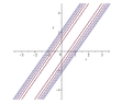
So far so good. So for k=1, I get two straight lines, one intersecting the y-axis at -1 and one at 1. Same for every other value of k. However, when I put k=0, I get y=2x.

Drawing the levels curves in both MAPLE and Wolfram Alpha, resulted in plots in which there is no line going through the origin. My question is why ? What am I missing about k=0 ?

Thank you !

View attachment 7945

 

[S.G. Janssens]

I think the issue is that for $k = 0$ the two solution branches of $f(x,y) := (y - 2x)^2 = k$ degenerate into one branch (line). In Maple, you can try something like

f := (x,y) -> (y - 2*x)^2:
eps := 0.05:
plots:-contourplot(f, -3..3, -3..3, contours = [eps, 1, 3]);

As you decrease the value of "eps", you will see the corresponding branches not only approach each other, but also their plots become worse and worse. (This can be partially compensated for by increasing the number of grid points using the "grid" option of the plotting command.) In the left figure we have eps = 0.05 and in the right figure we have eps = 0.025.

Note that if $(x_0,y_0)$ is a point on the contour corresponding to $k = 0$, then indeed $y_0 = 2x_0$ and both partial derivatives $D_xf(x_0,y_0)$ and $D_yf(x_0,y_0)$ vanish, so the implicit function theorem fails badly.

 

[johng1]

Here's some comments on drawing graphs of "implicit" functions. I don't know how WolframAlpha draws such, but probably it's similar to what I have done. To draw such a graph f(x,y) = 0, partition the rectangle of interest in the x-y plane into a bunch of "small" rectangles. In each small rectangle, look for a point $(x_0,y_0)$ satisfying the equation. Here, the equation of the tangent plane to z = f(x,y) at $(x_0,y_0)$ is very useful. Of course this tangent plane "normally" is found with the aid of the 2 first partial derivatives of f. However, if these two partials are 0, something else must be done to look for a solution in the rectangle. Such a "bad" point on the graph is called a singular point. This makes the drawing algorithm work much "harder" (slower). In any event, after a bunch of points are found in the small rectangles, conceptually one has a bunch of dots. Just connect the dots.

Here's a sequence of drawings that might be instructive. Each drawing is the graph of
$$\sin(\pi\sqrt{x^2+y^2})=c$$
First c=1/2, then c=0.99. These graphs are pairs of concentric circles with the distance between a pair of circles smaller as c gets larger. The last graph is when c=1. Here, every point on the graph is a singular point! Aside, I couldn't get WolframAlpha to draw this graph.

View attachment 7986

Here the "connect the dots" results in a poor drawing.View attachment 7987

Here's the same graph with only the dots plotted.

View attachment 7988

Make the mesh of the partition finer (more rectangles):

View attachment 7989

Finally, the graph of all singular points:

View attachment 7990