Energy of a particle in an Infinite square well?

In summary, the code uses the shooting method to find the energies of the bound states of a symmetric well.
  • #1
Homework Statement
We find the odd solutions from a python code, for odd results Wave_function returns 𝜓(0) .
And for even results we look for solutions where 𝜓′(0)=0 by returning psi[-1,1] from Wave_function.

After getting these results we are supposed to compare them to the results we would get from by solving the equation in Griffiths?
Relevant Equations
E = [ (n^2) (pi^2) (h-bar^2) ] / [ 2 * m * a^2]
Here are the results from the python code:
Odd results:
Odd Results.PNG


Even results:
Even Results.PNG


I tried to solve for energy using the equation:
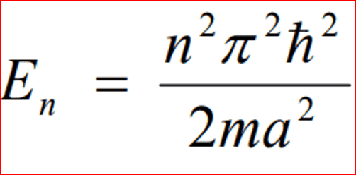
Equation.PNG

I substituted the value for a as 4, as in the code the limit goes from -a to a, rather then 0 to a, and hence in the code a = 2, but for the equation it would equal to 4. However after trying various values of n, none of my results are close to the ones obtained in the equation.
What am Idoing wrong?
How would I get something similar to the values obtained from the code?
 

Attachments

  • Odd Results.PNG
    Odd Results.PNG
    14.8 KB · Views: 131
Physics news on Phys.org
  • #2
Hello mighty @zeus8olympus, :welcome: !

zeus8olympus said:
Homework Statement:: We find the odd solutions from a python code
What code ? Your code, a package ? Please post using
[Code=Python]xyz[/Code]
Python:
xyz
and show what you are calling, and how
for odd results Wave_function returns 𝜓(0) .
And for even results we look for solutions where 𝜓′(0)=0 by returning psi[-1,1] from Wave_function.
 
  • #3
BvU said:
Hello mighty @zeus8olympus, :welcome: !


What code ? Your code, a package ? Please post using
[Code=Python]xyz[/Code]
Python:
xyz


Python:
from pylab import *
from scipy.integrate import odeint #A differential equation solver
from scipy.optimize import brentq #A root finding algorithm
import matplotlib.pyplot as plt
import numpy as np #An immensely useful library for manipulating arrays and lists (i.e matrices and vectors)

def V(x):
    global a #Means variable 'a' is available to any part of the code, thus we can set 'a' later and our V(x) will be aware of it.
    if abs(x) > a:
        return 100000
    else:
        return 0
        

def D1D2(psi, x):
    D1 = psi[1] #First derivative
    D2 = 2.0*(V(x) - E)*psi[0] #Second derivative
    return array([D1, D2])

def Wave_function(energy):
    global psi
    global E
    E = energy                #We need this so as to pass it to DD
    psi = odeint(D1D2, psi0, x)
    return psi[-1,0]
    
N = 10000                   # number of discrete points on the x-axis
a = 2                       # Set the width of the well
E = 0                       # initialize the global variable E
psi = np.zeros([N,2])       # Wave function values and its derivative (psi and psi')
psi0 = array([0,1])         # Wave function initial states
x = linspace(-a, 0, N)      # the points on the x-axis between left wall of the well and x=0
Emax = 100.0 
Ebottom = 0.0                # let us only look for solutions between Ebottom =0 and Emax=100
en = linspace(Ebottom, Emax, 1000) # A number of discrete energies where we will calculate psi(x=0)
psi_b = []                  # vector of wave function at x = 0 for all of the energies in en
for e1 in en:
    psi_b.append(Wave_function(e1))     # Determine psi(x=0) for every e1 in en
    
plt.plot(en, psi_b, 'r-')
plt.xlabel(r'$E$',size=20)
plt.ylabel(r'$\psi(x=0)$',size=20)
plt.grid(True)
plt.show()

def find_all_zeroes(x,y): #Returns list of values of x for which y(x)=0
    all_zeroes = []
    s = sign(y)
    for i in range(len(y)-1):
        if s[i]+s[i+1] == 0:
            zero = brentq(Wave_function, x[i], x[i+1])
            all_zeroes.append(zero)
    return all_zeroes
    
E_zeroes = find_all_zeroes(en, psi_b)   # now find the precise energies where psi(x=0) = 0 
print( "Energies for the bound states are: ")
for E in E_zeroes:
        print( '%11.7f' % E)
        
x = linspace(-a, a, N)
h=2*a/(N-1)
for E in E_zeroes[0:4]:
        Wave_function(E)
        psi[:,0]=psi[:,0]/sqrt(h*np.sum(np.square(psi[:,0])))
        plt.plot(x, psi[:,0], label="E = %.2f"%E)
        
plt.xlabel(r'$x$',size=20)
plt.ylabel(r'$\psi(x)$',size=20)
plt.legend()
plt.grid(True)
plt.show()

and show what you are calling, and how
From the question:
we will be solving the infinite symmetric well using what is called the shooting method. The potential does not need to be a square well to use this method, but it is important that it is symmetric. To make the potential symmetric we define the potential from −𝑎−a to 𝑎a whereas Griffiths has it from 00 to 𝑎a. Furthermore, we shall use units where ℏ2/𝑚=1ℏ2/m=1.
shoot.PNG
 
  • #4
Well, I'm not an expert at python, but after a lot of struggling I managed to get your results.
For the odd ##n## states it even prints nine 'energies' that rougly follow ##E_n = 0.353 \, n^2 ## where we expect ##E_n = 0.125 \, n^2 ##.

I didn't understand how $${\hbar ^2\over 2m} {\partial^2\over \partial x^2}\;\psi = (V-E)\;\psi $$ leads to
Python:
def D1D2(psi, x):
    D1 = psi[1] #First derivative
    D2 = 2.0*(V(x) - E)*psi[0] #Second derivative
    return array([D1, D2])
if ##{h^2\over 2m} = 1\;##. In other words: I miss a factor ##4\pi^2## ?

fumbled in the factor but didn't get the right answers yet:
Code:
Energies for the bound states are:
  0.0312500
  0.1250000
  0.2812500
  0.5000000
  0.7812500
  1.1250000
So a factor of 16 off from ##2 n^2\over 16##. Check normalization !
 
  • #5
Any news ?
 
  • #6
BvU said:
Any news ?
Sorry about the delay, i looked at what you said, and figured that when i was calculating the values i didnt factor h^2/2m as 1. but once i did so i got the same values as the code. and i got a perfect score as well. Thanks for the help.
 
  • Like
Likes vanhees71 and BvU

Suggested for: Energy of a particle in an Infinite square well?

Back
Top