MHB Fitting a function to a sinusoidal curve

[bugatti79]

Hi Folks,

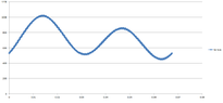
I have a curve that varies sinusoidally calculated from a numerical program as attached "Trace.png". I would like to fit this amplitude modulation expression to it.

f(t)=A[1+B \cos(\omega_1 t+ \phi)] \cos(\omega_2 t+ \theta)

I managed to adjust the parameters manually to get a very similar curve but couldn't exactly match it. Is there a mathematical technique I could use or is it possible at all?

Thanks

 

[Ackbach]

I would use Excel or LibreOffice Calc's Nonlinear Solver routine to solve this problem. Here's the setup:

Column A contains your time values.
Column B contains your data points.
Column C contains the various parameters you can vary, such as $A, B, \omega_1, \omega_2, \phi,$ and $\theta$.
Column D contains the formula you want to fit, all depending on values from Column C (you'll have to populate Column C with initial guesses). Don't forget to use, e.g.,

$C$1

to retrieve the value from C1.
Column E contains the square of the differences between Column B and Column D. Sum this column at the bottom.

That's the setup. Next, you invoke the Solver routine, and minimize the sum of squares at the bottom of Column E by varying the cells in Column C. If you're in LibreOffice Calc, you have to tell Calc to use a nonlinear solver, or else you'll get an error.

See if that works for you.

 

[bugatti79]

I would use Excel or LibreOffice Calc's Nonlinear Solver routine to solve this problem. Here's the setup:

Column A contains your time values.
Column B contains your data points.
Column C contains the various parameters you can vary, such as $A, B, \omega_1, \omega_2, \phi,$ and $\theta$.
Column D contains the formula you want to fit, all depending on values from Column C (you'll have to populate Column C with initial guesses). Don't forget to use, e.g.,

$C$1

to retrieve the value from C1.
Column E contains the square of the differences between Column B and Column D. Sum this column at the bottom.

That's the setup. Next, you invoke the Solver routine, and minimize the sum of squares at the bottom of Column E by varying the cells in Column C. If you're in LibreOffice Calc, you have to tell Calc to use a nonlinear solver, or else you'll get an error.

See if that works for you.

HI Ackbach

THanks, I will give it a go.

 

[bugatti79]

Hi Folks,

An additional idea cross my mind regarding the attachment "trace.png".

This curve comes from a numerical program which converts this trace to the frequency domain and plots all the harmonics $n_k \omega t$ and their amplitudes $a_n$, $b_n$.

What I would like to do is take these harmonics and their amplitudes and enter them into the Fourier series below to reproduce the same trace

x_t=d_0+d_1 \cos( n_1\omega t - \phi)+d_2 \cos( n_2\omega t - \phi)+d_3 \cos( n_3\omega t - \phi)+...

where $d_0=a_0/2$, $d_n=\sqrt (a_n^2+b_n^2)$ and $\phi_n=tan^{-1} (b_n/a_n)$

However, how would I determine $a_0$?