Inverse Discrete Laplace Transform

[swraman]

Hi,

I have an idea which when tested looks like its clearly flawed. I am hoping someone can tell me where my procedure is flawed, or point me to some other theory that has already done something similar.

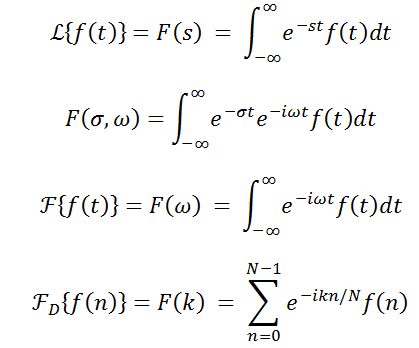
The first two are the laplace transform.
The third line is the Fourier Transform.
The last line is teh Discrete Fourier transform.

Im looking at lines 2 and 4 (along with how 3 - the Fourier transform is related to 4). Is there anything stopping me from modifying the Discrete Fourier transform by adding in an extra variable sigma to the loop - an exp(-sigma*n/N) term - and iterating over a range of sigmas. That is, each Sigma would result in one "DFT".

If I do this process with an input time function h(t) equal to the impulse response of a system - that is compute the "DFT" over a range of sigma's. Then, if I place each of these "DFT"s together into a surface plot, should it not look like the transfer function plot of the system (represented by impulse response h(t) )?

I would expect to see the magnitude of the "DFT"s to spike to infinity at the value of sigma and omega representing the poles of the system whose impulse response is h(t). I used a simple 2-DOF system to generate an impulse response, then ran this process across a range of sigmas (my natural frequency was well within my sampling parameters' capability). But as I said, the result doesn't look like I expected..

Is there something incorrect with my thinking here?

Thanks

 

[Orodruin]

Why would you do 2 and what do you think is new about it? It is just the continuation of the Laplace (or Fourier) transform to the complex plane...

 

[swraman]

I just added eqn (2) to show how similar the Laplace transform is to the Fourier transform (which has a well defined Discrete cousin in the DFT). I know there's nothing new about it.

The thinking was: If (4) is the discretized version of (3), why can we not generate another function that is a discretized version of (2) by adding in the extra exponential decay term into (4)?

 

[deskswirl]

What you have described is called the z-transform. But it does not parallel the Continuous Time Fourier Transform (CTFT) to Discrete Fourier Transform (DFT) relationship exactly. The DFT maps between two discrete domains corresponding to sampling of f(t) and F(ω). If one were to take the Discrete Time Fourier Transform (DTFT - note this is NOT the DFT!) which is a mapping of the sampled f(t) in the ω domain and then generalize it you would in fact have the Z-transform.