Parallel RLC circuit complex impedance graphing

[lys04]

Homework Statement

How can I graph the impedance against the frequency using a logarithmic scale for the frequency axis?

Relevant Equations

$$ Z = \frac{iwL-w^{2}RLC}{1-w^{2}LC+iwRC} $$

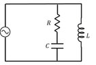
^^ as mentioned in the homework statement, the relevant equation is my worked out impedance for the circuit. I have attached a diagram of the circuit below.

 

[BvU]

https://en.wikipedia.org/wiki/Bode_plot

$\$

 

[lys04]

https://en.wikipedia.org/wiki/Bode_plot

$\$

Can you explain? I looked at it but I'm still confused

 

[BvU]

$Z$ is complex. You want to write it as $|Z| e^{j\phi}$. Do you know how to do that ?

$\$

 

[lys04]

$Z$ is complex. You want to write it as $|Z| e^{j\phi}$. Do you know how to do that ?

$\$

Is it like this? for the branch with resistor and capacitor,

And then for the branch with just the inductor in it its just wLe^90j?

And then I need to add them together which is 1/Z = 1/Z_l + 1/Z_c?

 

[BvU]

No. You already did the work to get the correct complex $Z$.

To write it as $|Z| e^{j\phi}$ you want to use $|Z|^2=ZZ^*$ with $Z^*$ the complex conjugate.
And $\tan\phi = \Im Z/\Re Z$ (imaginary part / real part).

If $Z= (a+jb)/(c+jd)$ you get the real and imaginary part by multiplying with $(c-jd)/(c-jd)$ (because then the denominator $c^2-d^2$ is real).

$\$

 

[kuruman]

If $Z= (a+jb)/(c+jd)$ you get the real and imaginary part by multiplying with $(c-jd)/(c-jd)$ (because then the denominator $c^2-d^2$ is real).

Did you mean to say "the denominator $c^2+d^2$ is real"?

 

[BvU]

Yes, thanks !

$\$

 

[FactChecker]

To actually make a graph, you will need values for R, L, and C. Then you can do the complex arithmetic and get Z(w) as a complex function of w. Then, |Z(w)| is the gain and arg(Z(w)) is the phase shift of the response. You can plot the result. A Bode plot does that.

 

[lys04]

To write it as |Z|ejϕ you want to use |Z|2=ZZ∗ with Z∗ the complex conjugate.
And tan⁡ϕ=ℑZ/ℜZ (imaginary part / real part).

If Z=(a+jb)/(c+jd) you get the real and imaginary part by multiplying with (c−jd)/(c−jd) (because then the denominator c2−d2 is real).

Alright,

I did

$$ \frac{iwL-w^{2}RLC}{1-w^2LC+iwRC} . \frac{1-w^2LC-iwRC}{1-w^2LC-iwRC}$$ which gives me $$ \frac{iwL-iw^3L^2C+w^4RL^2C^2+iw^2R^2C^2L}{(1-w^2LC)^2+(wRC)^2}$$

But this still has i's in it?

 

[lys04]

Alright,

I did

$$ \frac{iwL-w^{2}RLC}{1-w^2LC+iwRC} . \frac{1-w^2LC-iwRC}{1-w^2LC-iwRC}$$ which gives me $$ \frac{iwL-iw^3L^2C+w^4RL^2C^2+iw^2R^2C^2L}{(1-w^2LC)^2+(wRC)^2}$$

But this still has i's in it?

And also do I need to take square root to get |z|?

 

[kuruman]

You need to separate the real and imaginary parts first. This means find real numbers $Z_1$ and $Z_2$ such that $$Z=Z_1+iZ_2.$$ Then $$|Z|=\sqrt{Z_1^2+Z_2^2}.$$

 

[lys04]

To actually make a graph, you will need values for R, L, and C. Then you can do the complex arithmetic and get Z(w) as a complex function of w. Then, |Z(w)| is the gain and arg(Z(w)) is the phase shift of the response. You can plot the result. A Bode plot does that.

Yeah I have values of R, L and C given to me.

Is arg(z) $$ tan(\phi) = \frac{Im(Z)}{Re(Z)} $$?

 

[lys04]

You need to separate the real and imaginary parts first. This means find real numbers $Z_1$ and $Z_2$ such that $$Z=Z_1+iZ_2.$$ Then $$|Z|=\sqrt{Z_1^2+Z_2^2}.$$

Okay,

real part of |z|^2 is $$ \frac{w^4RL^2C^2}{(1-w^2LC^2)^{2}+(wRC)^{2}} $$ and imaginary part is $$ \frac{wL-w^3L^2C+w^3R^2C^2L}{(1-w^2LC^2)^{2}+(wRC)^{2}}$$

And then do I need to take the square root?

 

[lys04]

Okay,

real part of |z|^2 is $$ \frac{w^4RL^2C^2}{(1-w^2LC^2)+(wRC)^2}$$ and imaginary part is $$ \frac{wL-w^3L^2C+w^3R^2C^2L}{(1-w^2LC^2)+(wRC)^2}$$

And then do I need to take the square root?

Oh wait what I got above is z1^2 and z2^2 so then I just need to take the square root of their sum?

 

[kuruman]

Oh wait what I got above is z1^2 and z2^2 so then I just need to take the square root of their sum?

No.
If you have $$Z=\frac{iwL-iw^3L^2C+w^4RL^2C^2+iw^2R^2C^2L}{(1-w^2LC)^2+(wRC)^2},$$the real part is $$Z_1=\frac{w^4RL^2C^2}{(1-w^2LC)^2+(wRC)^2}$$and the imaginary part is $$Z_2=\frac{wL-w^3L^2C+w^2R^2C^2L}{(1-w^2LC)^2+(wRC)^2}.$$You need to find $$|Z|=\sqrt{Z_1^2+Z_2^2}.$$

 

[lys04]

No.
If you have $$Z=\frac{iwL-iw^3L^2C+w^4RL^2C^2+iw^2R^2C^2L}{(1-w^2LC)^2+(wRC)^2},$$the real part is $$Z_1=\frac{w^4RL^2C^2}{(1-w^2LC)^2+(wRC)^2}$$and the imaginary part is $$Z_2=\frac{wL-w^3L^2C+w^2R^2C^2L}{(1-w^2LC)^2+(wRC)^2}.$$You need to find $$|Z|=\sqrt{Z_1^2+Z_2^2}.$$

But is the first fraction you've got not |z|^2 since its ZZ*?

 

[lys04]

Alright I did it anyways, does this look correct?, using x for w

 

[FactChecker]

There are a few different ways to solve this. One way is how you are approaching it and another way is to convert it to a Laplace transformation. How are you supposed to solve this currently for your class?

 

[lys04]

There are a few different ways to solve this. One way is how you are approaching it and another way is to convert it to a Laplace transformation. How are you supposed to solve this currently for your class?

Using phasors I think

 

[FactChecker]

Using phasors I think

Then I think your work is good. The only "knit-pick" I would mention is that you might see if your graphics tool can directly plot x on a logarithmic scale and label it appropriately.

 

[lys04]

I'm trying to do this on python, neglect the fact that I'm plotting admittance instead, but why is the graph showing negative values? I don't think that's correct?

 

[lys04]

By the way the solutions look like this

 

[DaveE]

By the way the solutions look like this
View attachment 352416

It's much more clear on log-log plot, which is standard. That way you will get straight line asymptotes for an approximate solution. Pro EEs will call the vertical axis dBΩ, which is $20*log(|Z|)$, the phase is plotted as degrees, both with either a $log(\omega)$ or $log(f)$ horizontal axis.

You will want to keep your transfer function in a factored pole-zero form where you have linear $(1+\frac{ j \omega}{\omega_n})$, or quadratic $(1+(\frac{1}{Q})(\frac{ j \omega}{\omega_n}) + (\frac{ j \omega}{\omega_n})^2)$ terms. These will typically be separated in frequency and can thus be treated independently in the plotting process.

The correct (intuitive) way is really a lot to explain here, but look for this book online (I can't link to it here). It has a good description of manual frequency response (bode) plotting in section 8. You can pretty much ignore most all of the previous comments (sorry guys, I call them like I see them). Your original formula for Z in post #1 is all you need. Further arithmetic will just obscure things. You want the polynomial factors of $j \omega$, not the expanded polynomial. Do not simplify $(j \omega)^2 = -\omega^2$, even though that's true. That's great for a calculator, but not a good approach for understanding the system dynamics.

Finally, there is a big advantage to learning how to do this by hand for analog EEs. Even though your data lives in a computer that can calculate and plot things for you, you won't get a good understanding of what a pole, zero, or quadratic term really does to the frequency response of your system. It's similar to learning in your algebra class to solve quadratic equations even though Wolfram-Alpha et. al. can do it for you.

P.S. - In that book, as well as most other analog EE texts, you will see polynomials in $s$. For your case you can use $s=j \omega$, which is true for steady state solutions. You'll learn why people do this later (hint: Laplace Transforms).

 

[FactChecker]

$$ \frac{iwL-w^{2}RLC}{1-w^2LC+iwRC} . \frac{1-w^2LC-iwRC}{1-w^2LC-iwRC}$$ which gives me $$ \frac{iwL-iw^3L^2C+w^4RL^2C^2+iw^2R^2C^2L}{(1-w^2LC)^2+(wRC)^2}$$

In post #10, that last term should have $w^3$. That is corrected in post #14 and 18, but it led post #16 astray.

 

[vela]

But is the first fraction you've got not |z|^2 since its ZZ*?

You didn't calculate $ZZ^*$. You multiplied by 1 in a way to make the denominator real, so the expression you got is just another form of $Z$.

Another way you could have attacked this problem is to put both the numerator and denominator in polar form:

$$Z = \frac {a+bi}{c+di} = \frac{\sqrt{a^2+b^2}\,e^{i\varphi_1}}{\sqrt{c^2+d^2}\,e^{i\varphi_2}} = \underbrace{\sqrt\frac{a^2+b^2}{c^2+d^2}}_{\lvert Z \rvert}e^{i(\varphi_1-\varphi_2)}$$ where $\varphi_1 = \arg(a+bi)$ and $\varphi_2 = \arg(c+di)$.

Either way, you should get the same result. I think the second way involves less tedious algebra.

 

[DaveE]

You will want to keep your transfer function in a factored pole-zero form where you have linear $(1+\frac{ j \omega}{\omega_n})$, or quadratic $(1+(\frac{1}{Q})(\frac{ j \omega}{\omega_n}) + (\frac{ j \omega}{\omega_n})^2)$ terms. These will typically be separated in frequency and can thus be treated independently in the plotting process.

The correct (intuitive) way is really a lot to explain here, but look for this book online (I can't link to it here). It has a good description of manual frequency response (bode) plotting in section 8. You can pretty much ignore most all of the previous comments (sorry guys, I call them like I see them). Your original formula for Z in post #1 is all you need. Further arithmetic will just obscure things. You want the polynomial factors of $j \omega$, not the expanded polynomial. Do not simplify $(j \omega)^2 = -\omega^2$, even though that's true. That's great for a calculator, but not a good approach for understanding the system dynamics.

Oops! I failed to recheck your original equation. You'll want it in terms of $j \omega$ for easy analysis, like this: $$ Z(j \omega) =
j \omega L
\frac
{(1+ j \omega CR)}
{(1+j \omega CR) +( j \omega )^2 LC)} $$
This can also be expressed in the canonical form as
$$ Z(j \omega) =
j \omega L
\frac
{(1+(\frac{1}{Q}) (\frac{j \omega}{\omega_o}))}
{(1+(\frac{1}{Q}) (\frac{j \omega}{\omega_o}) +( \frac{j \omega}{\omega_o})^2 )} $$
Where $\omega_o = \frac{1}{\sqrt{LC}}$, $Q = \frac{Z_o}{R}$, and $Z_o = \sqrt{ \frac{L}{C} }$