Remusco
- 30
- 3
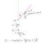
- Homework Statement
- I need to simulate a rotary inverted pendulum in Python for a school project. After about a week of struggling with this, I need help.
- Relevant Equations
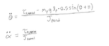
- # Compute accelerations using the equations of motion
alphaddot = tau_m / J_p # Motor arm angular acceleration
thetaddot = ((m_p * g * l / 2) * np.sin(theta[k-1]) + tau_p) / J_p #pendulum acceleration
[Mentor Note: Two threads on the same project have been merged into one]
I need serious help with this. I'm totally stuck as to why my results are mediocre. It would mean a ton if someone could at least point me in the right direction.
Below is my attempt:
I need serious help with this. I'm totally stuck as to why my results are mediocre. It would mean a ton if someone could at least point me in the right direction.
Below is my attempt:
import matplotlib.pyplot as pltimport numpy as npfrom scipy.integrate import solve_ivp# System Parametersm_p = 0.5 # Mass of the pendulum (kg)l = 0.4 # Length of the pendulum (m)r_a = 0.2 # Length of the motor-driven arm (m)g = 9.81 # Gravity (m/s^2)J_p = (1/3) * m_p * l**2 # Moment of inertia of the pendulum (rod pivoted at one end)# Motor ParametersV_supply = 18 # Motor supply voltage (V)R_motor = 9 # Motor resistance (Ohms)k_e = .1 # Back-EMF constant (V/(rad/s))k_t = .1 # Motor torque constant (Nm/A)# PID controller parameters for pendulumKp_pend, Ki_pend, Kd_pend = 10, 0, 0# PID controller parameters for motor armKp_arm, Ki_arm, Kd_arm = 5, 0, 0# Desired anglestheta_desired = 0 # Upright pendulum positionalpha_desired = np.radians(135) # Desired arm angle# Simulation Parameterst_sim = np.linspace(0, 20,800) # Time vectordt = t_sim[1] - t_sim[0]# Initialize State Variablestheta = np.zeros(len(t_sim)) # Pendulum anglethetadot = np.zeros(len(t_sim)) # Pendulum angular velocityalpha = np.zeros(len(t_sim)) # Motor arm anglealphadot = np.zeros(len(t_sim)) # Motor arm angular velocityu_control_signal = np.zeros(len(t_sim)) # Motor control signal PWM# Define initial conditionstheta[0], alpha[0] = np.radians(2), np.radians(270)thetadot[0], alphadot[0] = 0, 0# Initialize the PID Control Variables at 0integral_term_pend, derivative_term_pend = 0, 0integral_term_arm, derivative_term_arm = 0, 0# Previous error initializationprevious_theta_error = 0previous_alpha_error = 0# Simulation loopfor k in range(1, len(t_sim)): # Compute errors (desired - actual) theta_error = (theta_desired - theta[k-1]) alpha_error = (alpha_desired - alpha[k-1]) # PID control calculations for pendulum integral_term_pend += theta_error * dt derivative_term_pend = (theta_error - previous_theta_error) / dt u_pend = Kp_pend * theta_error + Ki_pend * integral_term_pend + Kd_pend * derivative_term_pend # PID control calculations for motor arm integral_term_arm += alpha_error * dt derivative_term_arm = (alpha_error - previous_alpha_error) / dt u_arm = Kp_arm * alpha_error + Ki_arm * integral_term_arm + Kd_arm * derivative_term_arm # Total control signal u_control_signal[k] = np.clip(u_pend + u_arm,-255,255) # Convert control signal (PWM) to motor voltage V_motor = (u_control_signal[k] / 255) * V_supply # Estimate motor current I_motor = (V_motor - k_e * alphadot[k-1]) / R_motor # Compute motor torque tau_m = k_t * I_motor # Compute pendulum torque from motor torque tau_p = (tau_m * l) / r_a # Compute accelerations using the equations of motion alphaddot = tau_m / J_p # Motor arm angular acceleration thetaddot = ((m_p * g * l / 2) * np.sin(theta[k-1]) + tau_p) / J_p # Pendulum angular acceleration # Update velocities and positions using Euler integration alphadot[k] = alphadot[k-1] + alphaddot * dt thetadot[k] = thetadot[k-1] + thetaddot * dt alpha[k] = alpha[k-1] + alphadot[k] * dt theta[k] = theta[k-1] + thetadot[k] * dt # Update previous errors previous_theta_error = theta_error previous_alpha_error = alpha_error# Plot Resultsplt.figure(figsize=(12, 6))# Plot Pendulum Angle Responseplt.subplot(2, 1, 1)plt.plot(t_sim, theta, label=r'$\theta$ (Pendulum Angle)')plt.plot(t_sim, alpha, label=r'$\alpha$ (Motor Arm Angle)')plt.axhline(y=0, color='gray', linestyle='dotted', label=r'$\theta = 0$ (Upright)')plt.xlabel('Time (s)')plt.ylabel('Angle (rad)')plt.title('PID-Controlled Pendulum Response')plt.legend()plt.grid(True)# Plot Control Signal (u)plt.subplot(2, 1, 2)plt.plot(t_sim, u_control_signal, label=r'$u$ (Motor Control Signal)', color='red')plt.xlabel('Time (s)')plt.ylabel('PWM Signal (u)')plt.title('Control Signal Output from PID Controller')plt.legend()plt.grid(True)plt.tight_layout()plt.show()
Last edited by a moderator: