Steven Thomas
- 16
- 0
Hi all,
I'm currently in the middle of performing an experiment for the final project of my MSc, and I have a question about how I should go about weighting the data when fitting a curve to it using the MATLAB fitting tool.
Firstly, a bit of background about the problem.
I am seeing how low temperature plasmas can be used to dissociate CO2, Carbon Dioxide, into CO, Carbon Monoxide. In order to see how much CO there is after the plasma I use an FTIR and absorption spectroscopy to measure the area of part of the spectra. I am currently trying to rerun the CO calibration.
To do this, I pass known admixtures of Argon and CO, then measure the area. So I have ten values of CO percentage, 0.1% to 1.0 percent in 0.1% increments, and I have 10 corresponding areas, each having been calculated from the mean of 10 readings at each admixture, so I also have a corresponding standard deviation (σ) and standard error (SE) for each admixture.
Normally I would just fit a function with the admixture along the x-axis and the area on the y axis, weighting each point with either 1/σ2 or 1/SE2. However, as in my experiment I will be recording areas of CO curves and want a corresponding percentage out, it is better for me to fit the data the other way around, with percentage along the y-axis and area on the x axis. With the data this way round I am fitting the function f(x) = a*x2 + b*x.
Without specifying any weights to my data points, I get the fit below:

with error on the coefficients as: a ±10.8%, and b ±13.4%.
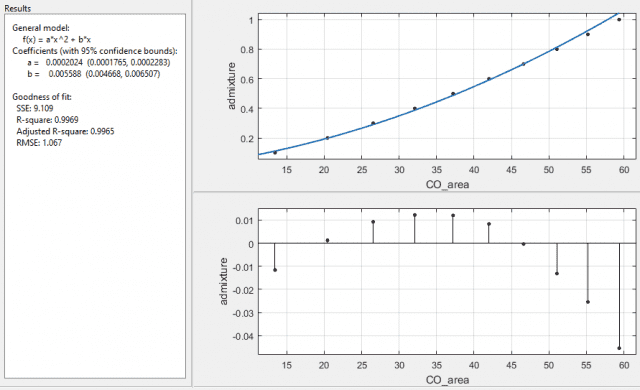
With 1/σ2 as the weights I get:

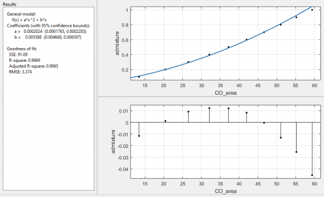
and with 1/SE2 I get:

both with error on the coefficients as a ±12.8%, and b ±16.5%. Interesting that the function it returns is the same, for the last two cases, with the same R-square and adjusted R-square values, but with different SSE and RMSE values. The SSE is a factor of 10 different and the RMSE is a factor of √10 different, which I assume is due to the 10 readings used for the means taken into account when using the standard error over the standard deviation. What I am a little puzzled about is why the fit is now worse when I've specified which data points it should more carefully plot to.
So finally I come to asking my question - why? Have I misinterpreted how to use the weighting function in matlab, and should I have lower numbers as the ones I want to fit more carefully to?
Or is it because I have flipped the axis round on my data, so if I was just to plot the data with error bars, they would now be horizontal rather than vertical?
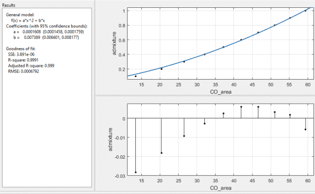
I am suspecting the second to be true, as I have tried fitting the function using just σ2 and SE2, and I get the following respectively:


again, both with the same values of the coefficients with errors a ±9.4%, and b ±10.7%. So the errors are lower, the SSE and RMSE are lower, and the R-square values are closer to 1 too.
Which way should I be doing it? Or have I got this all wrong and shouldn't be using absolute standard errors to weight with, but instead should be using percentage standard errors?
I know this is a bit of a long post, so if you've read this far I really thank you, but I've going through this for a couple of days now and would like some advice from someone better at statistics than I am.
Thanks in advance,
Steve.
I'm currently in the middle of performing an experiment for the final project of my MSc, and I have a question about how I should go about weighting the data when fitting a curve to it using the MATLAB fitting tool.
Firstly, a bit of background about the problem.
I am seeing how low temperature plasmas can be used to dissociate CO2, Carbon Dioxide, into CO, Carbon Monoxide. In order to see how much CO there is after the plasma I use an FTIR and absorption spectroscopy to measure the area of part of the spectra. I am currently trying to rerun the CO calibration.
To do this, I pass known admixtures of Argon and CO, then measure the area. So I have ten values of CO percentage, 0.1% to 1.0 percent in 0.1% increments, and I have 10 corresponding areas, each having been calculated from the mean of 10 readings at each admixture, so I also have a corresponding standard deviation (σ) and standard error (SE) for each admixture.
Normally I would just fit a function with the admixture along the x-axis and the area on the y axis, weighting each point with either 1/σ2 or 1/SE2. However, as in my experiment I will be recording areas of CO curves and want a corresponding percentage out, it is better for me to fit the data the other way around, with percentage along the y-axis and area on the x axis. With the data this way round I am fitting the function f(x) = a*x2 + b*x.
Without specifying any weights to my data points, I get the fit below:
with error on the coefficients as: a ±10.8%, and b ±13.4%.
With 1/σ2 as the weights I get:
and with 1/SE2 I get:
both with error on the coefficients as a ±12.8%, and b ±16.5%. Interesting that the function it returns is the same, for the last two cases, with the same R-square and adjusted R-square values, but with different SSE and RMSE values. The SSE is a factor of 10 different and the RMSE is a factor of √10 different, which I assume is due to the 10 readings used for the means taken into account when using the standard error over the standard deviation. What I am a little puzzled about is why the fit is now worse when I've specified which data points it should more carefully plot to.
So finally I come to asking my question - why? Have I misinterpreted how to use the weighting function in matlab, and should I have lower numbers as the ones I want to fit more carefully to?
Or is it because I have flipped the axis round on my data, so if I was just to plot the data with error bars, they would now be horizontal rather than vertical?
I am suspecting the second to be true, as I have tried fitting the function using just σ2 and SE2, and I get the following respectively:
again, both with the same values of the coefficients with errors a ±9.4%, and b ±10.7%. So the errors are lower, the SSE and RMSE are lower, and the R-square values are closer to 1 too.
Which way should I be doing it? Or have I got this all wrong and shouldn't be using absolute standard errors to weight with, but instead should be using percentage standard errors?
I know this is a bit of a long post, so if you've read this far I really thank you, but I've going through this for a couple of days now and would like some advice from someone better at statistics than I am.
Thanks in advance,
Steve.