Leonid92
- 45
- 2
I wrote the following code in MATLAB:
Thus I generated data whose behavior is described by equation y = a*exp(-t/b)+c, with adding some noise. Then I fit mentioned function to these data and found values of parameters:
The plot of simulated data and fit is below:
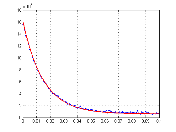
One person told me that it would be good to consider this problem in logarithmic scale. Could you please tell me, what is usually implied when talking about transforming ordinary plot to logarithmic scale? How should I implement this procedure? Should I first convert my simulated y-values into log-scale and after that perform fit with another function? What formulas should I use? Is it reasonable to use logarithm with base 10 or logarithm with base 'e'?
I will be very appreciate for any help or advice.
P.S. Unfortunately, I don't have opportunity to ask that person in more detail regarding this question.
Code:
t = [0:0.001:0.1];
noise = randn(1,size(t,2));
a = 15*10^9;
b = 15*10^(-3);
c = 7*10^8;
y = a*exp(-t/b)+c+noise*100000000;
fun = @(p,t)p(1)*exp(-t/p(2))+p(3);
p0 = [15.5*10^9, 14*10^(-3), 6*10^8];
p = lsqcurvefit(fun, p0, t, y);
t_fit = [0:0.0001:0.1];
y_fit = fun(p,t_fit);
fig = figure('Visible','on');
plot(t,y,'.');
hold on;
grid on;
plot(t_fit,y_fit,'r','linewidth',2);
disp(sprintf('a=%d; b=%.4f; c=%d',p(1),p(2),p(3)))
Code:
a=1.550000e+10; b=0.0149; c=6.000000e+08One person told me that it would be good to consider this problem in logarithmic scale. Could you please tell me, what is usually implied when talking about transforming ordinary plot to logarithmic scale? How should I implement this procedure? Should I first convert my simulated y-values into log-scale and after that perform fit with another function? What formulas should I use? Is it reasonable to use logarithm with base 10 or logarithm with base 'e'?
I will be very appreciate for any help or advice.
P.S. Unfortunately, I don't have opportunity to ask that person in more detail regarding this question.
Attachments


