- #1
xzyan
- 6
- 0
Hello everyone, I'm new here and new to Matlab. I hope I do place the post in the right place.
First of all, thanks for viewing my post. Please bear with my English. I tried my best to explain everything clear. If you have any question about anything I wrote or spot any fault, please tell me. Many thanks!
1. The problem statement
The problem is to use Matlab to modelling the 3-level rate equation of a solid-state laser.

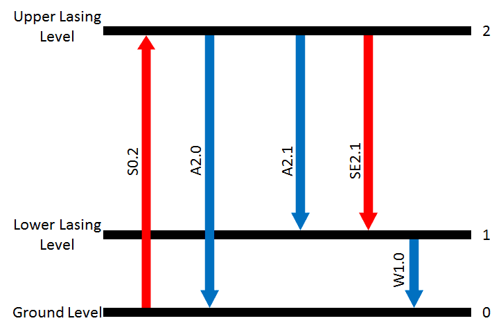
The picture shows the simplified energy levels and transitions of the laser.
S0.2 is the absorption from ground level (L0) to upper lasing level (L2).
A2.0 is the spontaneous emission from upper lasing level (L2) to ground level (L0).
A2.1 is the spontaneous emission from upper lasing level (L2) to lower lasing level (L1).
SE2.1 is the stimulated emission from upper lasing level (L2) to lower lasing level (L1).
W1.0 is the fast non-radiative decay from lower lasing level (L1) to ground level (L0).
In this problem, the absorption S0.2 is triggered by pump laser source with intensity of Ip, stimulated emission SE2.1 is triggered by signal laser source with intensity of Is.
I did write a MATLAB function with a main script to do the modelling. However, the MATLAB keeps running for a long time and no output is obtained. (I've tried run it on the server for 3 days) I did try a simplified 2 level system with only one beam (i.e. the pump only), and I got the results in about half an hour.
I was thinking, is it because of the solving function I was using is not suitable for this problem? (I'm using ODE45)
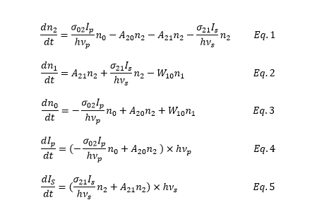
I've written down the rate equations according to the energy levels and transitions like follows:

where n2, n1 and n0 are the populations of the state in upper lasing level (L2), lower lasing level (L1) and ground level (L0), respectively. σ02 and σ21 are the absorption and stimulation emission cross section of S0.2 and SE2.1 transitions. A20 and A21 is the Einstein coefficient of transition A2.1 and A2.0. W10 is the rate of the fast transition W1.0. h is the Planck's constant, vp and vs are the frequencies of the pump laser and signal laser. Ip and Is are the intensities of the pump and signal laser.
The main idea of this modelling is to observe the change of the population of the state in each level and the change of the intensity of both the pump and signal lasers.
I have written a Matlab code as below:
Function
function dy = rate_eq( t,y )
%Simplfied rate equation for Yb ions. Detailed equation is in Mini-thesis
dy = zeros(5,1);
h = 6.62606957E-34;
% Planck constant (m^2kg/s)
c = 299792458;
% Speed of light (m/s)
lambdaS = 1030;
% Wavelength of signal light (nm)
lambdaP = 975;
% Wavelength of pump light (nm)
vS = c/lambdaS;
% Frequency of signal (Hz)
vP = c/lambdaP;
% Frequency of pump (Hz)
A21 = 1/(600E-6);
% Spontaneous emission transition time from L2 -> L1 of 600 us
A20 = 1/(600E-6);
% Spontaneous emission transition time from L2 -> L1 of 600 us
W10 = 1/(500E-12);
% Fast decay transition time from L1 -> L0 of 500 ps
sigma21 = 0.5E-20;
% Stimulation emission cross section from L2 -> L1 of 0.5E-20 cm^2
sigma02 = 2.5E-20;
% Absorption cross section from L0 -> L2 of 2.5E-20 cm^2
dy(1) = sigma02*y(4)*y(3)/(h*vP)-A20*y(1)-A21*y(1)-sigma21*y(5)*y(1)/(h*vS)
% Change of population of upper lasing level (L2)
dy(2) = A21*y(1)+sigma21*y(5)*y(1)/(h*vS)-W10*y(2)
% Change of population of lower lasing level (L2)
dy(3) = -sigma02*y(4)*y(3)/(h*vP)+A20*y(1)+W10*y(2)
% Change of population of ground lasing level (L2)
dy(4) = (-sigma02*y(4)*y(3)/(h*vP)+A20*y(1))*(h*vP)
% Change of intensity of pump beam
dy(5) = (sigma21*y(5)*y(1)/(h*vS)+A21*y(1))*(h*vS)
% Change of intensity of signal beam
end
Main Script
TSPAN = [0 1];
Y0 =[0 0 8.75E20 1 0.2];
%y(1) = population of Upper Lasing level
%y(2) = population of Lower Lasing level
%y(3) = population of Ground Level
%y(4) = Optical intensity of Pump W/cm^2
%y(5) = Optical intensity of Signal W/cm^2
[T,Y] = ode45(@rate_eq,TSPAN,Y0);
subplot(3,1,1)
plot(T,Y(:,3),T,Y(:,2),T,Y(:,1))
legend('Ground level','Lower lasing level','Upper lasing level')
title('Population different levels')
subplot(3,1,2)
plot(T ,Y(:,4))
title('Pump Intensiry') % Pump intensity
subplot(3,1,3)
plot(T ,Y(:,5))
title('Singal Intensity') % Signal intensity
Thanks again for your patience and kindly help!
First of all, thanks for viewing my post. Please bear with my English. I tried my best to explain everything clear. If you have any question about anything I wrote or spot any fault, please tell me. Many thanks!
1. The problem statement
The problem is to use Matlab to modelling the 3-level rate equation of a solid-state laser.
The picture shows the simplified energy levels and transitions of the laser.
S0.2 is the absorption from ground level (L0) to upper lasing level (L2).
A2.0 is the spontaneous emission from upper lasing level (L2) to ground level (L0).
A2.1 is the spontaneous emission from upper lasing level (L2) to lower lasing level (L1).
SE2.1 is the stimulated emission from upper lasing level (L2) to lower lasing level (L1).
W1.0 is the fast non-radiative decay from lower lasing level (L1) to ground level (L0).
In this problem, the absorption S0.2 is triggered by pump laser source with intensity of Ip, stimulated emission SE2.1 is triggered by signal laser source with intensity of Is.
Homework Equations
I did write a MATLAB function with a main script to do the modelling. However, the MATLAB keeps running for a long time and no output is obtained. (I've tried run it on the server for 3 days) I did try a simplified 2 level system with only one beam (i.e. the pump only), and I got the results in about half an hour.
I was thinking, is it because of the solving function I was using is not suitable for this problem? (I'm using ODE45)
The Attempt at a Solution
I've written down the rate equations according to the energy levels and transitions like follows:
where n2, n1 and n0 are the populations of the state in upper lasing level (L2), lower lasing level (L1) and ground level (L0), respectively. σ02 and σ21 are the absorption and stimulation emission cross section of S0.2 and SE2.1 transitions. A20 and A21 is the Einstein coefficient of transition A2.1 and A2.0. W10 is the rate of the fast transition W1.0. h is the Planck's constant, vp and vs are the frequencies of the pump laser and signal laser. Ip and Is are the intensities of the pump and signal laser.
The main idea of this modelling is to observe the change of the population of the state in each level and the change of the intensity of both the pump and signal lasers.
I have written a Matlab code as below:
Function
function dy = rate_eq( t,y )
%Simplfied rate equation for Yb ions. Detailed equation is in Mini-thesis
dy = zeros(5,1);
h = 6.62606957E-34;
% Planck constant (m^2kg/s)
c = 299792458;
% Speed of light (m/s)
lambdaS = 1030;
% Wavelength of signal light (nm)
lambdaP = 975;
% Wavelength of pump light (nm)
vS = c/lambdaS;
% Frequency of signal (Hz)
vP = c/lambdaP;
% Frequency of pump (Hz)
A21 = 1/(600E-6);
% Spontaneous emission transition time from L2 -> L1 of 600 us
A20 = 1/(600E-6);
% Spontaneous emission transition time from L2 -> L1 of 600 us
W10 = 1/(500E-12);
% Fast decay transition time from L1 -> L0 of 500 ps
sigma21 = 0.5E-20;
% Stimulation emission cross section from L2 -> L1 of 0.5E-20 cm^2
sigma02 = 2.5E-20;
% Absorption cross section from L0 -> L2 of 2.5E-20 cm^2
dy(1) = sigma02*y(4)*y(3)/(h*vP)-A20*y(1)-A21*y(1)-sigma21*y(5)*y(1)/(h*vS)
% Change of population of upper lasing level (L2)
dy(2) = A21*y(1)+sigma21*y(5)*y(1)/(h*vS)-W10*y(2)
% Change of population of lower lasing level (L2)
dy(3) = -sigma02*y(4)*y(3)/(h*vP)+A20*y(1)+W10*y(2)
% Change of population of ground lasing level (L2)
dy(4) = (-sigma02*y(4)*y(3)/(h*vP)+A20*y(1))*(h*vP)
% Change of intensity of pump beam
dy(5) = (sigma21*y(5)*y(1)/(h*vS)+A21*y(1))*(h*vS)
% Change of intensity of signal beam
end
Main Script
TSPAN = [0 1];
Y0 =[0 0 8.75E20 1 0.2];
%y(1) = population of Upper Lasing level
%y(2) = population of Lower Lasing level
%y(3) = population of Ground Level
%y(4) = Optical intensity of Pump W/cm^2
%y(5) = Optical intensity of Signal W/cm^2
[T,Y] = ode45(@rate_eq,TSPAN,Y0);
subplot(3,1,1)
plot(T,Y(:,3),T,Y(:,2),T,Y(:,1))
legend('Ground level','Lower lasing level','Upper lasing level')
title('Population different levels')
subplot(3,1,2)
plot(T ,Y(:,4))
title('Pump Intensiry') % Pump intensity
subplot(3,1,3)
plot(T ,Y(:,5))
title('Singal Intensity') % Signal intensity
Thanks again for your patience and kindly help!
