Differentials in Multivariable Functions ....

In summary, Peter needs help understanding an example in Chapter 2 of Shmuel Kantorovitz's book "Several Real Variables". Kantorovitz declares that the ratio ##\frac{ \mid \phi_0(h) \mid }{ \| h \| } ( h \neq 0 )## is bounded as ##h \rightarrow 0##. However, Peter does not see how to apply this to the limit as h approaches 0. Apologies if I'm being slow.
  • #1
Math Amateur
Gold Member
MHB
3,990
48
I am reading the book "Several Real Variables" by Shmuel Kantorovitz ... ...

I am currently focused on Chapter 2: Derivation ... ...

I need help with an aspect of Kantorovitz's Example 4 on page 66 ...

Kantorovitz's Example 4 on page 66 reads as follows:
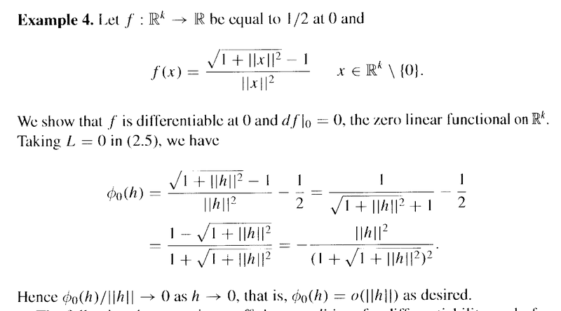
Kantorovitz - Example 4 ...  Page 66 ...  ... .png

In the above example, Kantorovitz shows that##\phi_0 (h) = - \frac{ \| h \|^2 }{( 1 + \sqrt{ 1 + \| h \|^2 )}^2 }##Kantorovitz then declares that ## \frac{ \phi_0 (h) }{ \| h \| } \rightarrow 0## as ##h \rightarrow 0## ... ...Can someone please show me how to demonstrate rigorously that this is true ... that is that
## \frac{ \phi_0 (h) }{ \| h \| } \rightarrow 0## as ##h \rightarrow 0## ... ...
Help will be much appreciated ...

Peter============================================================================================

***NOTE***

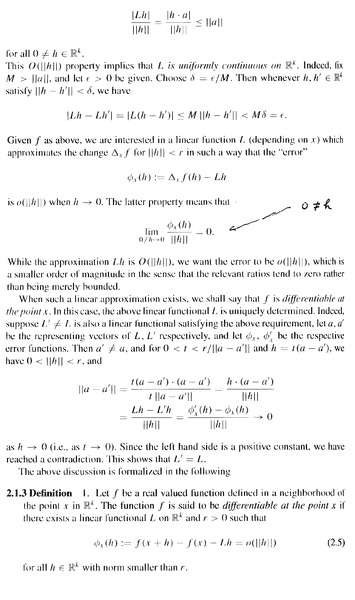
Readers of the above post may be helped by having access to Kantorovitz' Section on "The Differential" ... so I am providing the same ... as follows:
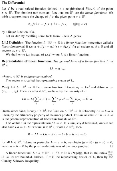
Kantorovitz - 1 - Sectiion on the DIfferential ... PART 1 ... .png

Kantorovitz - 2 - Sectiion on the DIfferential ... PART 2 ... .png

Kantorovitz - 3 - Sectiion on the DIfferential ... PART 3 ... .png
Hope that helps readers understand the context and notation of the above post ,,, ,,,

Peter
 

Attachments

  • Kantorovitz - Example 4 ...  Page 66 ...  ... .png
    Kantorovitz - Example 4 ... Page 66 ... ... .png
    18.8 KB · Views: 853
  • Kantorovitz - 1 - Sectiion on the DIfferential ... PART 1 ... .png
    Kantorovitz - 1 - Sectiion on the DIfferential ... PART 1 ... .png
    27.4 KB · Views: 437
  • Kantorovitz - 2 - Sectiion on the DIfferential ... PART 2 ... .png
    Kantorovitz - 2 - Sectiion on the DIfferential ... PART 2 ... .png
    34.9 KB · Views: 427
  • Kantorovitz - 3 - Sectiion on the DIfferential ... PART 3 ... .png
    Kantorovitz - 3 - Sectiion on the DIfferential ... PART 3 ... .png
    13.2 KB · Views: 416
Last edited:
Physics news on Phys.org
  • #2
##\phi_0(h) = \mathcal O(h^2)## implies that ##\phi_0(h)/h=\mathcal O(h)##.
 
  • #3
Orodruin said:
##\phi_0(h) = \mathcal O(h^2)## implies that ##\phi_0(h)/h=\mathcal O(h)##.
Thanks for the reply Orodruin ...

BUT ... don't quite follow ... and do not see how to apply to the limit ...

Apologies if I'm being slow ...

PeterEdit: I do know that ##O( \| h \| ) \Longrightarrow## the ratios ##\frac{ \mid \phi_0(h) \mid }{ \| h \| } ( h \neq 0 )## are bounded ...
 
  • #4
Math Amateur said:
Thanks for the reply Orodruin ...

BUT ... don't quite follow ... and do not see how to apply to the limit ...

Apologies if I'm being slow ...

PeterEdit: I do know that ##O( \| h \| ) \Longrightarrow## the ratios ##\frac{ \mid \phi_0(h) \mid }{ \| h \| } ( h \neq 0 )## are bounded ...
You can think of ##f(x)=O(g(x))## as ##f(x) \leq c\cdot g(x)## for some constant ##c##.

E.g. if ##f(h)=c_1{h^2}+c_2{h^3}+c_3{h^4}+\ldots ## for small ## h > 0##, then we can assume ##h < 1## and ##h^2 > h^3 > h^4 >\ldots## which means ## f(h) \leq (\sum c_i) h^2##. So if the coefficients don't outnumber the behavior of ##{h}##, i.e. if ##\sum c_i = c## is finite, then we get ##f(h) \leq c \cdot h^2## which we write as ##f(h)=O(h^2).## In this case however, we also have ##\frac{1}{h}f(h) < c\cdot h## and thus ##\frac{f(h)}{h} =O(h)\,.##

A simple example for its usage is the matrix exponent. The question is about algorithms: How many multiplications of input variables are necessary to multiply two ##(n \times n)## matrices?

The ordinary way is to do it by ##n^3## multiplications. Improved algorithms can do it with ##c \cdot n^\gamma## multiplications (above some fixed ##n## where the improvement starts to be one) and ##\gamma## is somewhere above ##2## and of course below ##3## and ##c## a constant independent of ##n##. The matrix algorithm then goes by ##O(n^\gamma)## essential multiplications. The infimum of these ##\gamma## is called the matrix exponent ##\omega ##, but this only as a side note. For short people say: matrix multiplication goes by ##O(n^\omega)##. IIRC multiplication of ##2 \times 2## matrices which are usually done by eight multiplications can be done by only seven at the cost of additional additions, which shows ##\omega < 3##.

The example above, ##f(h)=O(h^2)## means, that ##f(h)## doesn't grow faster than a constant multiple of ##h^2\,.##
One of my favorite jokes is to write constants as ##O(1)##.
 
  • Like
Likes Math Amateur

What is a multivariable function?

A multivariable function is a mathematical function that depends on two or more variables. This means that the output of the function is determined by the values of multiple independent variables.

What is a differential in a multivariable function?

A differential in a multivariable function is the change in the output of the function with respect to a specific variable. It is a measure of how the output of the function changes as one of the variables changes.

Why are differentials important in multivariable functions?

Differentials allow us to study how the output of a multivariable function changes in response to changes in its input variables. This is important for understanding the behavior of complex systems and making predictions based on mathematical models.

How do you calculate differentials in multivariable functions?

To calculate the differential of a multivariable function, you need to take the partial derivatives of the function with respect to each of its input variables. These partial derivatives can then be combined to form the total differential of the function.

What are some real-world applications of differentials in multivariable functions?

Differentials in multivariable functions are used in many areas of science and engineering, such as physics, economics, and finance. They are particularly useful in modeling systems with multiple variables, such as weather patterns, economic markets, and chemical reactions.

Similar threads

Replies
3
Views
1K
Replies
2
Views
1K
Replies
2
Views
1K
Replies
8
Views
2K
Replies
3
Views
1K
Replies
2
Views
2K
  • Topology and Analysis
Replies
4
Views
2K
Replies
1
Views
913
  • Topology and Analysis
Replies
2
Views
966
Back
Top