Estimate \theta with Importance Sampling: Plot Convergence vs Sample Size

[Jameson]

Problem:

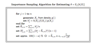
Use importance sampling to estimate the quantity:

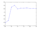
\(\displaystyle \theta = \int_{0}^{\infty}x \frac{e^{-(y-x)^2/2}e^{-3x}}{Z}dx\), where \(\displaystyle Z=\int_{0}^{\infty}e^{-(y-x)^2/2}e^{-3x}dx\) and $y=0.5$. Plot the converge of the estimator versus sample size. Note: You may consider $3e^{-3x}$ as the density for importance sampling.

Attempt:

This is a new topic that I digesting but as far as I understand it, this technique is used to reduce variance in Monte Carlo estimation and has a much faster convergence for small values. For example, if we want to estimate the $P[X>5]$ if $X$ is a standard normal random variable, then it will take a very large amount of samples to get this value so it's not practical.

If we are trying to estimate \(\displaystyle \theta=\int f(x)g(x)dx\) we can rewrite this as \(\displaystyle \int \frac{f(x)g(x)}{h(x)}h(x)dx\)

This problem appears to take a similar form but I'm not sure what my first step is. According to my notes I should be trying find $\hat{\theta}$ by the following:

\(\displaystyle \hat{\theta}=\frac{1}{n} \sum_{i=1}^{n}\frac{f(X_i)g(X_i)}{h(X_i)}\).

Can anyone provide some insight into the idea here or tips to get started?

 

[I like Serena]

To be honest, I'm unfamiliar with importance sampling.
But we can see how far we can get.

Let's start with your integrals: it seems you have a typo in them - they do not converge!
Can it be that it should be for instance $-(y-x)^2$ instead of $(-y-x)^2$?

 

[Jameson]

You're quite right. Good catch. Will edit after posting this.

So I know that I need to start with generating random variables that follow the distribution $3e^{-3x}$. I believe this can be done in Matlab by the command since $3e^{-3x}$ is the pdf for an exponential random variable with mean 3.

x=exprnd(-3)

 

[I like Serena]

You're quite right. Good catch. Will edit after posting this.

So I know that I need to start with generating random variables that follow the distribution $3e^{-3x}$. I believe this can be done in Matlab by the command since $3e^{-3x}$ is the pdf for an exponential random variable with mean 3.

x=exprnd(-3)

Looks good. :)

As I understand it, if you have a distribution with pdf(x), then:
$$\mathbb E_{pdf}[g(x)] = \int g(x)pdf(x) dx$$
It can be estimated by:
$$\hat{\mathbb E}_{pdf}[g(x)] = \frac 1 n \sum_{i=1}^n g(x_i)$$
where $\{x_i\}$ is a set of random samples that is distributed with pdf(x).

So this is something we should already be able to do.

 

[Jameson]

Definitely. If I want to use the classical Monte Carlo method to estimate $E[g(X)]$ where each $X_i$ follows an exponential distribution then I would do something like:

X=exprnd(1,10000,1);
g=X.^2;
E=mean(g);

The above assumes that $g(x)=x^2$ and $x$ follows an exponential distribution with mean 1. It will average 10000 samples to approximate the expected value.

It's going from this to the new theory though that's confusing me. I'm reading up on http://www.columbia.edu/~mh2078/MCS04/MCS_var_red2.pdf article now from Columbia University. I'll try to post if anything comes out of it.

EDIT: I suppose if I can figure out what my $h(x), g(x), f(x)$ are then this will straightforward.

 

[I like Serena]

Definitely. If I want to use the classical Monte Carlo method to estimate $E[g(X)]$ where each $X_i$ follows an exponential distribution then I would do something like:

X=exprnd(1,10000,1);
g=X.^2;
E=mean(g);

The above assumes that $g(x)=x^2$ and $x$ follows an exponential distribution with mean 1. It will average 10000 samples to approximate the expected value.

It's going from this to the new theory though that's confusing me. I'm reading up on http://www.columbia.edu/~mh2078/MCS04/MCS_var_red2.pdf article now from Columbia University. I'll try to post if anything comes out of it.

EDIT: I suppose if I can figure out what my $h(x), g(x), f(x)$ are then this will straightforward.

Yep!

I think the catch is that the approximation will tend to break down since the exponential distribution is so asymmetric, causing most samples to be in the low range and samples in the high range will not be representative.
That's why they introduce extra functions to switch to another pdf that picks up on more of the "important" samples.

 

[Jameson]

I agree and the idea makes sense in principle but I can't yet do it in practice. I am stuck on figuring out what is what with the expression \(\displaystyle \frac{e^{-(y-x)^2/2}e^{-3x}}{Z}\).

I also don't know if I should try to simplify this analytically before running a simulation or just plug in each $X_i$ into $\displaystyle \hat{\theta}=\frac{1}{n} \sum_{i=1}^{n}\frac{f(X_i)g(X_i)}{h(X_i)}$ directly.

Here are the steps from the Columbia paper I'm reading. It seems they advocate directly plugging in each $X_i$ but again I don't know what my $h,f,g$ are.

View attachment 1663

I think I'll try working on another problem for a bit and come back to this to see if any new ideas stir.

 

[I like Serena]

I agree and the idea makes sense in principle but I can't yet do it in practice. I am stuck on figuring out what is what with the expression \(\displaystyle \frac{e^{-(y-x)^2/2}e^{-3x}}{Z}\).

I also don't know if I should try to simplify this analytically before running a simulation or just plug in each $X_i$ into $\displaystyle \hat{\theta}=\frac{1}{n} \sum_{i=1}^{n}\frac{f(X_i)g(X_i)}{h(X_i)}$ directly.

Here are the steps from the Columbia paper I'm reading. It seems they advocate directly plugging in each $X_i$ but again I don't know what my $h,f,g$ are.

View attachment 1663

I think I'll try working on another problem for a bit and come back to this to see if any new ideas stir.

As I understand it, you are supposed to evaluate the integral:
$$I \underset{def}{=} \int x \frac{\phi(x; 0.5) \epsilon(x; 3)}{Z}dx$$
where $\phi(x;y)$ is the pdf of the normal distribution with mean $y$, $\epsilon(x; \lambda)$ is pdf of the exponential distribution with parameter $\lambda$, and $Z$ is the normalization constant for the pdf in the numerator.Let's pick $f(x) = x$ and $g(x) = \frac{\phi(x; 0.5) \epsilon(x; 3)}{Z}$.
Then g(x) is a pdf, since it is normalized (integral of g(x) is 1).

So:
$$I = E_g[X] = E_g[f(X)] = E_\epsilon[f(X)g(X)/\epsilon(X; 3)] = E_\epsilon[X \cdot \phi(X;0.5)]$$

You can try to estimate it with the distribution $g(X)$, with the distribution $\epsilon(X, 3)$, or even with the distribution $\phi(x;0.5)$. One will probably be more accurate than another...

 

[Jameson]

Interesting.

If we have $g(x) = \frac{\phi(x; 0.5) \epsilon(x; 3)}{Z}$ then computing the larger integral seems bad this way because first we have to estimate $Z$ then we need to estimate the larger integral. That sounds like running a Monte Carlo inside a Monte Carlo.

From this line:

$I = E_g[X] = E_g[f(X)] = E_\epsilon[f(X)g(X)/\epsilon(X; 3)] = E_\epsilon[X \cdot \phi(X;0.5)]$

It seems like there are two options for a density function, $g$ and $\epsilon$. Out of those two I can easily generate random variables that follow an exponential distribution so I'd pick that one if I had to choose.

The steps seem to be:

1) Generate a large enough number of random samples following some distribution.
2) Plug in each $X_i$ into other expressions
3) Average expressions for final estimate

(1) is doable although I still don't see how to go to (2). Forgive me as this post is kind of repeating things I've already written but these concepts are still sinking in.

 

[I like Serena]

If we have $g(x) = \frac{\phi(x; 0.5) \epsilon(x; 3)}{Z}$ then computing the larger integral seems bad this way because first we have to estimate $Z$ then we need to estimate the larger integral. That sounds like running a Monte Carlo inside a Monte Carlo.

Actually, you can rewrite Z to the cdf of the normal distribution (complete the square).
Matlab can calculate the result for you.

From this line:

It seems like there are two options for a density function, $g$ and $\epsilon$.

Actually, you can also pick $\phi$, which Matlab will support.

I do not know yet which you should choose, but I guess you can try them all.

Out of those two I can easily generate random variables that follow an exponential distribution so I'd pick that one if I had to choose.

The steps seem to be:

1) Generate a large enough number of random samples following some distribution.
2) Plug in each $X_i$ into other expressions
3) Average expressions for final estimate

(1) is doable although I still don't see how to go to (2). Forgive me as this post is kind of repeating things I've already written but these concepts are still sinking in.

I don't understand.
If you have an $X_i$, can't you simply plug it in the formula that you've chosen?
Like you did before?

And I think you should create an array with random samples.
Then pick only the first m samples for an estimation with m samples, where m=1, ..., n.
That way you can plot the estimation of the integral versus the sample size.
I think the problem statement is asking for that.

 

[Jameson]

Actually, you can rewrite Z to the cdf of the normal distribution (complete the square).
Matlab can calculate the result for you.

Ok let's try this first.

\(\displaystyle \begin{array}{}
e^{-(y-x)^2/2}e^{-3x}
& =e^{-(y^2-2xy+x^2)/2}e^{-3x} \\
&=e^{-(y^2-2xy+x^2+6x)/2}\\
&=e^{-(1/4-x+x^2+6x)/2} \\
&=e^{-(1/4+x^2+5x)/2} \\
\end{array}\)

On the right track? The CDF of a normal distribution has the form of \(\displaystyle \frac{1}{\sqrt{2\pi}} \int_{-\infty}^{x}\text{exp}(-t^2/2)dt\) so I'm not sure I can get to that form. From here Wolfram can't factor it so I've made a mistake or something isn't working... maybe you mean the pdf? Or maybe the constant terms in the cdf's for the numerator and the denominator cancel?

Actually, you can also pick $\phi$, which Matlab will support.

I do not know yet which you should choose, but I guess you can try them all.

I definitely intend to! I need to know this theory well for an upcoming quiz. :)

I don't understand.
If you have an $X_i$, can't you simply plug it in the formula that you've chosen?
Like you did before?

And I think you should create an array with random samples.
Then pick only the first m samples for an estimation with m samples, where m=1, ..., n.
That way you can plot the estimation of the integral versus the sample size.
I think the problem statement is asking for that.

Plug into what is the question. If I can manipulate the $g(x)$ you proposed into things that are workable in Matlab then I can plug in each $X_i$ easily.

 

[I like Serena]

Ok let's try this first.

\(\displaystyle \begin{array}{}
e^{-(y-x)^2/2}e^{-3x}
& =e^{-(y^2-2xy+x^2)/2}e^{-3x} \\
&=e^{-(y^2-2xy+x^2+6x)/2}\\
&=e^{-(1/4-x+x^2+6x)/2} \\
&=e^{-(1/4+x^2+5x)/2} \\
\end{array}\)

On the right track? The CDF of a normal distribution has the form of \(\displaystyle \frac{1}{\sqrt{2\pi}} \int_{-\infty}^{x}\text{exp}(-t^2/2)dt\) so I'm not sure I can get to that form. From here Wolfram can't factor it so I've made a mistake or something isn't working... maybe you mean the pdf? Or maybe the constant terms in the cdf's for the numerator and the denominator cancel?

Yep. That is the right direction.
You need something of the form:
$$e^{-(x-a)^2 / 2 + b} = e^b \cdot e^{-(x-a)^2 / 2}$$
Then substitute:
$$t = x - a$$

 

[Jameson]

Ok so moving forward then I need to factor: $1/4+x^2+5x$. Taking the coefficient in front of $x$, dividing by 2 and squaring we get $\frac{1}{4}+x^2+5x+\frac{25}{4}-\frac{25}{4}=\left(x+\frac{5}{2} \right)^2-6$

So, \(\displaystyle e^{-(1/4+x^2+5x)/2} =e^{-3} \cdot e^{\frac{(x+5/2)^2}{2}}\)...

I don't know what the $t=x-a$ substitution will help with in calculation but I assume from here I should try to rewrite the original problem. Before I can do that I still don't know how we account for the fact that we don't have a $\frac{1}{\sqrt{2\pi}}$. There is a $\phi$ in the numerator and we are claiming there is one too in the denominator. Is that why it doesn't need to be there?

 

[I like Serena]

Ok so moving forward then I need to factor: $1/4+x^2+5x$. Taking the coefficient in front of $x$, dividing by 2 and squaring we get $\frac{1}{4}+x^2+5x+\frac{25}{4}-\frac{25}{4}=\left(x+\frac{5}{2} \right)^2-6$

So, \(\displaystyle e^{-(1/4+x^2+5x)/2} =e^{-3} \cdot e^{\frac{(x+5/2)^2}{2}}\)...

Looks good!
... but I think you lost a minus somewhere...

I don't know what the $t=x-a$ substitution will help with in calculation but I assume from here I should try to rewrite the original problem. Before I can do that I still don't know how we account for the fact that we don't have a $\frac{1}{\sqrt{2\pi}}$. There is a $\phi$ in the numerator and we are claiming there is one too in the denominator. Is that why it doesn't need to be there?

You have:
$$Z = \int_0^\infty e^{-(y-x)^2/2}e^{-3x} dx = \int_0^\infty e^{3} \cdot e^{-\frac{(x+5/2)^2}{2}} dx$$

And you also have:
$$\Phi(u) = \frac 1 {\sqrt{2\pi}} \int_{-\infty}^u e^{-t^2/2} dt$$
where $\Phi$ is the standard normal cdf, which is a standard function in matlab.In other words:
$$Z = e^{3} \cdot \int_0^\infty e^{-\frac{(x+5/2)^2}{2}} dx$$
and:
$$\int_{a}^b e^{-t^2/2} dt = \sqrt{2\pi}\Big(\Phi(b) - \Phi(a)\Big)$$

Combine them?

 

[Jameson]

I'll try my best. My brain is melting. This is always how it seems to go though - first day I'm about to crack, second day it seems less crazy... xth day I get it. :)

Let's start with \(\displaystyle t=x-\left(-\frac{5}{2} \right)\)

So $Z$ becomes \(\displaystyle \int_0^\infty e^{3} \cdot e^{-\frac{(t)^2}{2}} dt=\sqrt{2\pi}(\Phi(\infty)-\Phi(0))=\sqrt{2\pi} \Big(1-\Phi(0) \Big)\)?

Plug that into Matlab then back substitute?

 

[I like Serena]

I'll try my best. My brain is melting. This is always how it seems to go though - first day I'm about to crack, second day it seems less crazy... xth day I get it. :)

Let's start with \(\displaystyle t=x-\left(-\frac{5}{2} \right)\)

So $Z$ becomes \(\displaystyle \int_0^\infty e^{3} \cdot e^{-\frac{(t)^2}{2}} dt=\sqrt{2\pi}(\Phi(\infty)-\Phi(0))=\sqrt{2\pi} \Big(1-\Phi(0) \Big)\)?

Plug that into Matlab then back substitute?

Almost.
The range of the integral changes after the substitution.
Since x runs from 0 to $\infty$, t will run from $\frac 5 2$ to $\infty$.
Otherwise you wouldn't need matlab, since \(\displaystyle \Phi(0) = \frac 1 2\).

Edit: Oh, and you lost an $e^{3}$.

 

[Jameson]

Almost.
The range of the integral changes after the substitution.
Since x runs from 0 to $\infty$, t will run from $\frac 5 2$ to $\infty$.
Otherwise you wouldn't need matlab, since \(\displaystyle \Phi(0) = \frac 1 2\).

Ah yes. That makes sense.

Ok so now we have analytically solved the integral as follows:

$\displaystyle Z=\int_{0}^{\infty}e^{-(y-x)^2/2}e^{-3x}dx =\int_0^\infty e^{3} \cdot e^{-\frac{(x+5/2)^2}{2}} dx= e^3 \int_{5/2}^{\infty}e^{-\frac{(t)^2}{2}} dt=e^3 \sqrt{2\pi} \big(1-\Phi(5/2) \big)$

exp(3)*(sqrt(2*pi)*(1-normcdf(2.5)))= 0.3126

The above is the result according to Matlab. Let's see what Wolfram says. It's the same! I love it when math works :D

Ok, so now I think I can test out the whole thing:

1) Generate exponential random variables with mean 3.

2) Plug them into \(\displaystyle \frac{\phi(x; 0.5) \epsilon(x; 3)}{0.3126}\)

3) Take the mean

I'll do that now but I think somehow this is actually the normal Monte Carlo method since we didn't really transform the integral... not sure though. No actually this doesn't seem right at now to me. Hopefully we're close.

EDIT: Maybe this form you mentioned is the one to try: \(\displaystyle E_\epsilon[f(X)g(X)/\epsilon(X; 3)]\)

I'm going to type up notes on this and go to my professor tomorrow for some clarification. Thank you so much ILS for your help! (Clapping)

 

[Jameson]

Some followup to this: I met with my professor this morning and we talked for a bit. He showed me this code to work with, which is what he is looking for.

clearn=round(10.^(1:0.5:6));

for k=1:length(n)
    x = exprnd(1/2,1,n(k));
    tn(k) = mean(x.*exp(-(0.5-x).^2/2)/3);
    td(k)= mean(exp(-(0.5-x).^2/2)/3);
    r(k) = tn(k)/td(k);
end

semilogx(n,r,'b-o')

So basically it seems that we first multiply and divide by 3, which gives us $3e^{-3x}$ as part of the expression, which we'll use as the density. Then what's left over is:

\(\displaystyle x\frac{e^{-(0.5-x)^2/2)}}{3}\)

I guess for a similar reason this expression disappears in $Z$. Still trying to digest it all but getting closer.

 

[I like Serena]

Some followup to this: I met with my professor this morning and we talked for a bit. He showed me this code to work with, which is what he is looking for.

clearn=round(10.^(1:0.5:6));

for k=1:length(n)
    x = exprnd(1/2,1,n(k));
    tn(k) = mean(x.*exp(-(0.5-x).^2/2)/3);
    td(k)= mean(exp(-(0.5-x).^2/2)/3);
    r(k) = tn(k)/td(k);
end

semilogx(n,r,'b-o')

So basically it seems that we first multiply and divide by 3, which gives us $3e^{-3x}$ as part of the expression, which we'll use as the density. Then what's left over is:

\(\displaystyle x\frac{e^{-(0.5-x)^2/2)}}{3}\)

I guess for a similar reason this expression disappears in $Z$. Still trying to digest it all but getting closer.

Let's take it apart.

We get a vector $(x_i)$ of $n_k$ random values from the exponential distribution with pdf $\frac 1 2 e^{-\frac 1 2 x}$.

The numerator is:
$$tn = \frac 1{n_k} \sum_{i=1}^{n_k} x_i \cdot e^{-(0.5-x_i)^2/2} \cdot \frac 1 3$$
This is an approximation for:
$$tn \approx \int_0^\infty x \cdot e^{-(0.5-x)^2/2} \cdot \frac 1 3 \cdot \frac 1 2 e^{-\frac 1 2 x} dx$$

But that does not look right.
That is not what you would need for the problem in your problem statement.
This is a different integral with a different exponential distribution.
(Never mind the constant factor, which is taken care of separately.)
Seems to me the exponential distribution in the first step should be with mean 3 instead of 1/2. Perhaps your professor intended for you to figure that out, since this would be for a different problem.

Then the denominator is:
$$td = \frac 1{n_k} \sum_{i=1}^{n_k} e^{-(0.5-x_i)^2/2} \cdot \frac 1 3$$
This is an approximation for:
$$td \approx \int_0^\infty e^{-(0.5-x)^2/2} \cdot \frac 1 3 \cdot \frac 1 2 e^{-\frac 1 2 x} dx$$
It is a second Monte Carlo method to find the constant Z! ;)

Actually, the constant is off, but since we're normalizing anyway, that's not a problem, as long as we are off by the same constant in numerator and denominator.

In other words, I think the code for your problem statement should be:

clear
n = round(10.^(1:0.5:6));

for k=1:length(n)
    x = exprnd(3,1,n(k));
    tn(k) = mean(x.*exp(-(0.5-x).^2/2));
    td(k)= mean(exp(-(0.5-x).^2/2));
    r(k) = tn(k)/td(k);
end

semilogx(n,r,'b-o')

Or, even better:

clear
n = round(10.^(1:0.5:6));
Z = exp(3)*(sqrt(2*pi)*(1-normcdf(2.5)));

for k=1:length(n)
    x = exprnd(3,1,n(k));
    r(k) = mean(x.*exp(-(0.5-x).^2/2)/Z);
end

semilogx(n,r,'b-o')

 

[Jameson]

I had a big typo, it should be:

x = exprnd(1/3,1,n(k));

So sorry!

Now, why is it 1/3 instead of 3? I originally thought the code should have 3 instead of 1/3 but I was reminded that if an exponential random variable takes the form of $\lambda e^{-\lambda x}$ then it has a mean of $\frac{1}{\lambda}$. In Matlab the code for generating an exponential random variable is:

exprnd(mu,# of rows in generated matrix, # of columns in generated matrix)

I've run your code you suggested with the change from $3 \rightarrow 1/3$ as explained and I get a different result than the fixed code from my professor. Here's how I modified your code:

clear
n = round(10.^(1:0.5:6));
Z = exp(1/3)*(sqrt(2*pi)*(1-normcdf(2.5)));

for k=1:length(n)
    x = exprnd(1/3,1,n(k));
    r(k) = mean(x.*exp(-(0.5-x).^2/2)/Z);
end

figure(2)
semilogx(n,r,'b-o')

I will be reviewing this more tonight so this is preliminary, but those are my initial comments.

 

[I like Serena]

Now, why is it 1/3 instead of 3? I originally thought the code should have 3 instead of 1/3 but I was reminded that if an exponential random variable takes the form of $\lambda e^{-\lambda x}$ then it has a mean of $\frac{1}{\lambda}$.

Aha!

I get a different result than the fixed code from my professor. Here's how I modified your code:

clear
n = round(10.^(1:0.5:6));
Z = exp(1/3)*(sqrt(2*pi)*(1-normcdf(2.5)));

for k=1:length(n)
    x = exprnd(1/3,1,n(k));
    r(k) = mean(x.*exp(-(0.5-x).^2/2)/Z);
end

figure(2)
semilogx(n,r,'b-o')

That should be:

Z = exp(3)*(sqrt(2*pi)*(1-normcdf(2.5)));

 

[Jameson]

Ok we're getting closer. Now your suggestion and my professor's differ by about a factor of 3. This might be due to the original note he made in this problem that we should consider $3e^{-3x}$ to be the density from which we generate variables. Since this "3" is missing, we must multiply and divide by it as to not change our original expression.

However, to argue against myself a bit I notice that in my professor's code we have these two lines:

 tn(k) = mean(x.*exp(-(0.5-x).^2/2)/3);
td(k)= mean(exp(-(0.5-x).^2/2)/3);

It seems as if the 1/3 in each part should cancel out. Thinking some more now...

 

[I like Serena]

Ok we're getting closer. Now your suggestion and my professor's differ by about a factor of 3. This might be due to the original note he made in this problem that we should consider $3e^{-3x}$ to be the density from which we generate variables. Since this "3" is missing, we must multiply and divide by it as to not change our original expression.

However, to argue against myself a bit I notice that in my professor's code we have these two lines:

tn(k) = mean(x.*exp(-(0.5-x).^2/2)/3);
td(k)= mean(exp(-(0.5-x).^2/2)/3);

It seems as if the 1/3 in each part should cancel out. Thinking some more now...

True. Looking at the original problem statement again, there is no 3 in it, so we should indeed compensate by a factor 1/3.
That factor should still be added to the calculation of r(k) in the code I suggested.
We did calculate the correct Z, so that does explain the difference of a factor 3.

Final code (with a small optimization):

clear
n = round(10.^(1:0.5:6));
Z = exp(3)*(sqrt(2*pi)*(1-normcdf(2.5)));

for k=1:length(n)
    x = exprnd(1/3,1,n(k));
    r(k) = mean(x.*exp(-(0.5-x).^2/2))/(3*Z);
end

figure(2)
semilogx(n,r,'b-o')

 

[Jameson]

(Clapping)

Well done ILS. You've taken a topic you hadn't seen before and had very poor guidance over from myself, and gave sound advice at every corner. I thank you again.

Just so you see here is the output of your code. It is 100% correct from everything I can tell. :)

clear
n = round(10.^(1:0.5:6));
Z = exp(3)*(sqrt(2*pi)*(1-normcdf(2.5)));

for k=1:length(n)
    x = exprnd(1/3,1,n(k));
    r(k) = mean(x.*exp(-(0.5-x).^2/2))/(3*Z);
end

figure(2)
semilogx(n,r,'b-o')

Output:

View attachment 1665

 

[I like Serena]

Good!

And here's W|A's result, which is 0.322745.

It does seem to match. ;)