Integral Calculus Tutorial

[Ackbach]

1. Prerequisites

In order to study integral calculus, you must have a firm grasp of differential calculus. You can go to

http://mathhelpboards.com/calculus-10/differential-calculus-tutorial-1393.html

for my differential calculus tutorial, although, of course, there are many books and other tutorials available as well. Note that the prerequisites I listed in my tutorial for differential calculus still apply. That is, integral calculus builds on and assumes differential calculus and all its prerequisites. So you still need your http://www.mathhelpboards.com/f2/algebra-dos-donts-1385/, geometry, and http://www.mathhelpboards.com/f12/trigonometry-memorize-trigonometry-derive-35/.

I already did an overview of integral calculus in the differential calculus tutorial, so I won't repeat it here. We'll just dive right in.

2. Area Under a Curve

From geometry, you should know how to compute areas of circles, rectangles, trapezoids, and other simple figures. But what is the area under the sine curve from $0$ to $\pi$? You won't learn that in geometry. The answer happens to be $2$. How did I get that?

2.1 Area Approximations

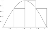
You can approximate the area under a curve by drawing a whole bunch of rectangles and adding up those areas. Let me illustrate: suppose we take our function $y=\sin(x)$, and take the interval $[0,\pi]$ and divide it up into four equal width sections. So we have $[0,\pi/4), [\pi/4,\pi/2), [\pi/2,3\pi/4),$ and $[3\pi/4,\pi]$. For each of these intervals, we draw a rectangle whose width is the width of the interval ($\pi/4$ for all four smaller intervals), and whose height is determined by the height of our function at the left-hand end of the interval. Here's a picture to illustrate:

https://www.physicsforums.com/attachments/322._xfImport

The left-most rectangle has no height because $\sin(0)=0$. So, what is the area of all those boxes? Well, we have a rather simple computation to make:

$$A\approx \sin(0)*( \pi/4)+ \sin( \pi/4)*( \pi/4)+ \sin( \pi/2)*( \pi/4)+ \sin(3 \pi/4)*( \pi/4)$$
$$=( \pi/4) \left(0+ \frac{\sqrt{2}}{2}+1+ \frac{\sqrt{2}}{2} \right)$$
$$= \frac{ \pi}{4} (1+\sqrt{2})$$
$$ \approx 1.896.$$

Not too bad (the percent error is $100 \% \cdot(2-1.896)/2 \approx 5.2\%$.)

We're studying math. Surely we get can a better answer than this! The answer I just gave is just fine for many situations, especially in engineering, but we'd like to know the exact answer if we can get it. Patience! The answer is coming.

Let's divvy up the interval into more than 4 sub-intervals - for grins let's do 10 subintervals. So the sum we need to compute now is
$$A \approx \frac{\pi}{10} \left( \sin(0)+ \sin(\pi/10)+ \sin(2\pi/10)+ \sin(3\pi/10)+ \dots + \sin(8\pi/10)+\sin(9\pi/10) \right).$$
You can see here that I've factored out the interval width, $\pi/10$, since all the intervals are the same width. You can always do that if the intervals are the same width. So, what do we get for this expression? You can plug this expression laboriously into your calculator, and come up with the decimal approximation $1.984$. That's closer, as it has the percent error $0.8\%$. Much better. But still not exact.

How do we get the exact number? Answer: by taking the limit as the number of rectangles goes to infinity. To do this conveniently, we need to introduce summation notation.

2.2 Summation Notation

No one wants to write out every term in a summation of the kind we've been talking about. It's cumbersome enough with only 10 terms. What if we had 100? Surely there's a way to write this summation in a compact form? Yes, there is. You use the capital Greek letter "sigma", written $\sum$, to express a summation. A summation typically has what's called a "dummy variable" whose value changes from one term in the summation to the next. Here's the way you write a summation:
$$\sum_{ \text{dummy variable}= \text{start}}^{ \text{finish}} \text{summand}.$$
As usual, the best way to illustrate is with examples. I'll start with an easy one:
$$\sum_{j=1}^{10}1=\underbrace{ \overbrace{1}^{j=1}+ \overbrace{1}^{j=2}+ \overbrace{1}^{j=3}+ \dots+ \overbrace{1}^{j=10}}_{10\; \text{times}}=10.$$
Here's a slightly harder one:
$$\sum_{j=1}^{10}j=\overbrace{1}^{j=1}+ \overbrace{2}^{j=2}+ \overbrace{3}^{j=3}+ \dots+ \overbrace{10}^{j=10}=55.$$
Interesting anecdote about this sum: Gauss supposedly figured out how to do this sum when he was a youngster and was punished, along with his class, by having to add up all the numbers from 1 to 1000. He reasoned that $1+1000=1001$, $2+999=1001$, $3+998=1001$, and so on. He paired a low number with a high number, and brought the values together. So how many pairs were there? $1000/2=500$. So the answer to the sum is $500*1001=500500$. That is,
$$\sum_{j=1}^{n}j=\frac{n(n+1)}{2}.$$
Homework: does this formula work when $n$ is odd?

Even harder:
$$\sum_{j=1}^{10}j^{2}=\overbrace{1}^{j=1}+ \overbrace{4}^{j=2}+ \overbrace{9}^{j=3}+ \dots+ \overbrace{100}^{j=10}=385.$$
There is a formula for this sum as well:
$$\sum_{j=1}^{n}j^{2}=\frac{n(n+1)(2n+1)}{6}.$$
You can prove this using mathematical induction.

Important facts about summation notation:

1. The dummy variable has no visibility outside the summation. Suppose I have an expression like this:
$$\sum_{j=1}^{10} \sin(j \pi)+\frac{e^{x}}{x}.$$
The $e^{x}/x$ doesn't know that the $j$ exists. So the scope of the $j$ is merely in the summation.

2. The exact identity of the dummy variable is unimportant. I could just as easily use $k$ as $j$:
$$\sum_{j=1}^{10}j=\sum_{k=1}^{10}k.$$
Remember: once I get outside the summation, no one knows about the dummy variable, so it doesn't matter what I use for dummy variables. This should make sense, since once I'm outside the summation, all I see are numbers, no dummy variable.

3. Summation is linear. This means two things:
$$\sum_{j=a}^{b}c\,f(j)=c\sum_{j=a}^{b}f(j),$$
and
$$\sum_{j=a}^{b}[f(j)+g(j)]=\sum_{j=a}^{b}f(j)+\sum_{j=a}^{b}g(j).$$
That this is true simply stems from the fact that addition is linear - then you prove this result using mathematical induction again.

2.3 Exact Value of Previous Area

Now that we are armed with summation notation, we can at least write our former sum compactly:
$$A\approx \frac{\pi}{10} \sum_{j=0}^{9} \sin(j\pi/10).$$
But we want more and more rectangles! What would this sum look like if we left the number of rectangles to be arbitrary? We'd get
$$A \approx \frac{\pi}{n} \sum_{j=0}^{n-1} \sin(j\pi/n).$$
How do you evaluate this sum? Well, if you look at the trig identity page on wiki, you'll see that there's a formula for exactly this sort of sum. That is, we have that
$$ \sum_{j=0}^{n} \sin( \varphi+j \alpha)= \frac{ \sin \left( \frac{(n+1) \alpha}{2} \right) \cdot \sin \left( \varphi+ \frac{n \alpha}{2} \right)}{ \sin( \alpha/2)}.$$
Whew! In our case, we can simplify this a bit. Comparing these two expressions, we see right away that $\varphi=0$. That leaves us with
$$ \sum_{j=0}^{n} \sin(j \alpha)= \frac{ \sin \left( \frac{(n+1) \alpha}{2} \right) \cdot \sin \left( \frac{n \alpha}{2} \right)}{ \sin( \alpha/2)}.$$
Now we don't want this sum to go all the way to $n$, but to $n-1$. So, just replace as follows:
$$ \sum_{j=0}^{n-1} \sin(j \alpha)= \frac{ \sin \left( \frac{n \alpha}{2} \right) \cdot \sin \left( \frac{(n-1) \alpha}{2} \right)}{ \sin( \alpha/2)}.$$
Finally, we see that we need $\alpha=\pi/n$. So, putting that in our expression yields
$$ \sum_{j=0}^{n-1} \sin(j \pi/n)=
\frac{ \sin \left( \frac{n ( \pi ) } { 2n } \right) \cdot \sin \left( \frac { (n-1) \pi } { 2n } \right) }
{ \sin( \pi / ( 2n ) ) }=
\frac{ \sin \left( \frac{ \pi } { 2 } \right) \cdot \sin \left( \frac { (n-1) \pi } { 2n } \right) }
{ \sin( \pi / ( 2n ) ) }=
\frac{ \sin \left( \pi / 2 - \pi / (2n) \right) } { \sin( \pi / ( 2n ) ) }.$$
We can use the addition of angle formula for the numerator to obtain
$$ \sum_{j=0}^{n-1} \sin(j \pi/n) = \frac{ \sin ( \pi/2 ) \cos( \pi/(2n)) - \sin(\pi/(2n)) \cos( \pi/2) } { \sin( \pi / ( 2n ) ) } = \frac{ \cos( \pi/(2n)) } { \sin( \pi / ( 2n ) ) }.$$
Yes, I could write the cotangent here, but I'm going to leave it where it is. So, to recap:
$$ \frac{ \pi}{n} \sum_{j=0}^{n-1} \sin(j\pi/n) = \frac{ \pi}{n} \frac{ \cos( \pi/(2n)) } { \sin( \pi / ( 2n ) ) }.$$
What we really want to do is compute the limit:
$$\lim_{n\to \infty} \frac{ \pi}{n} \sum_{j=0}^{n-1} \sin(j\pi/n) = \lim_{n\to \infty}\frac{ \pi}{n} \frac{ \cos( \pi/(2n)) } { \sin( \pi / ( 2n ) ) }.$$
So, what's going on in this limit is that the number of rectangles is going to infinity, and they are getting really small in width. Really small! We say they are getting infinitesimally small. Can we compute this limit? I think we can. Recall that
$$\lim_{x\to 0}\frac{\sin(x)}{x}=1.$$
Here's the dirty trick: I say that taking a limit as $n\to\infty$ is the same as saying that $(1/n)\to 0$. So, let's make the substitution $x=1/n$, and re-evaluate:
$$\lim_{n\to \infty}\frac{ \pi}{n} \frac{ \cos( \pi/(2n)) } { \sin( \pi / ( 2n ) ) }=
\lim_{x\to 0}(x\pi) \frac{ \cos( x \pi/2) } { \sin( x \pi / 2 ) }.$$
Quick, while no one's looking, I'm going to multiply and divide by $2$, thus:
$$=2\lim_{x\to 0}\frac{x\pi}{2} \frac{ \cos( x \pi/2) } { \sin( x \pi / 2 ) }.$$
Now I'm going to break this limit up into two pieces by using my product rule for limits:
$$=2\lim_{x\to 0}\frac{x\pi/2}{\sin(x\pi/2)}\cdot\lim_{x\to 0}\cos(x\pi/2).$$
If $x\to 0$, then surely $x\pi/2 \to 0$. And I can use quotient rules for limits to achieve
$$=2\frac{1}{\lim_{x\pi/2\to 0}\frac{\sin(x\pi/2)}{x\pi/2}}\cdot 1=2\cdot 1=2.$$
And there it is! The exact answer. No sweat, right? (I hope you were sweating through all that, actually, because it helps you to realize just how difficult a problem it is to find exact areas.)

 

[Ackbach]

Integral Calculus Tutorial Post 2 Draft

Comments and questions should be posted here:

http://mathhelpboards.com/commentary-threads-53/commentary-integral-calculus-tutorial-4229.html

2.4 Exact Value of Another Area

In the http://www.mathhelpboards.com/f10/differential-calculus-tutorial-1393/, Section 2.2, I mentioned as an example the area under the curve $f(x)=-x^{2}+2$ from $-\sqrt{2}$ to $\sqrt{2}$. Can we find this area exactly? Let's try. We need to form a summation expression, using our handy-dandy summation notation, that expresses the area approximation using an arbitrary number of rectangles. Build it up using 4 rectangles to start:
$$A\approx \frac{2\sqrt{2}}{4}\left(f(-\sqrt{2})+f(-\sqrt{2}+1\cdot 2\sqrt{2}/4)+f(-\sqrt{2}+2\cdot 2\sqrt{2}/4)+f(-\sqrt{2}+3\cdot 2\sqrt{2}/4)\right).$$
You can see that I'm using left-hand rectangles again. Let's try writing this in summation notation:
$$A\approx \frac{2\sqrt{2}}{4}\sum_{j=0}^{3}f(-\sqrt{2}+j\cdot 2\sqrt{2}/4).$$
Now, hopefully, you'll see that we can fairly easily write this for $n$ rectangles thus:
$$A\approx \frac{2\sqrt{2}}{n}\sum_{j=0}^{n-1}f(-\sqrt{2}+j\cdot 2\sqrt{2}/n).$$
Let's see if we can simplify this a bit. First, we plug in what $f$ is:
$$A\approx \frac{2\sqrt{2}}{n}\sum_{j=0}^{n-1}\left[-(-\sqrt{2}+j\cdot 2\sqrt{2}/n)^{2}+2\right]
=\frac{2\sqrt{2}}{n}\sum_{j=0}^{n-1}\left[-(2-j\cdot 8/n+j^{2}8/n^{2})+2\right]$$
$$=\frac{2\sqrt{2}}{n}\sum_{j=0}^{n-1}\left[\frac{8j}{n}-\frac{8j^{2}}{n^{2}}\right].$$
We can evaluate this sum! Note that $n$ does not change as the sum is written out, only the dummy variable $j$ does. Hence, we can rewrite, using the linearity of summations, as
$$A\approx \frac{2\sqrt{2}}{n}\left[\sum_{j=0}^{n-1}\frac{8j}{n}-\sum_{j=0}^{n-1}\frac{8j^{2}}{n^{2}}\right]=
\frac{2\sqrt{2}}{n}\left[\frac{8}{n}\sum_{j=0}^{n-1}j-\frac{8}{n^{2}}\sum_{j=0}^{n-1}j^{2}\right].$$
We can evaluate the summations at the right there by simply plugging $n-1$ into the formulas I mentioned above in the first post. That is, we get
\begin{align*}A&\approx \frac{2\sqrt{2}}{n}\left[\frac{8}{n}\cdot \frac{n(n-1)}{2}-\frac{8}{n^{2}}\cdot\frac{n(n-1)(2n-1)}{6}\right]\\
&=\frac{2\sqrt{2}}{n}\left[4(n-1)-\frac{4}{n}\cdot\frac{2n^{2}-3n+1}{3}\right]\\
&=2\sqrt{2}\left[4\left(1-\frac{1}{n}\right)-\frac{4}{3}\left(2-\frac{3}{n}+\frac{1}{n^{2}}\right)\right].
\end{align*}
I've gotten it into this form, because the expression $1/n$ or $1/n^{2}$ is particularly easy to evaluate in the limit as $n\to\infty$, which is what we want to do in order to get the exact area. So let's do that:
$$A=\lim_{n\to\infty}2\sqrt{2}\left[4\left(1-\frac{1}{n}\right)-\frac{4}{3}\left(2-\frac{3}{n}+\frac{1}{n^{2}}\right)\right]=2\sqrt{2}(4-8/3)=2\sqrt{2}(4/3)=\frac{8\sqrt{2}}{3}.$$
That's an exact area. If you're doing this problem for an engineering professor, however, he'd probably want a decimal approximation of $3.77$.

Hope you're sweating even more now. This is not the easy way to find areas under curves! There is a much better way: the Fundamental Theorem of the Calculus. However, in order to show you what that is, I'm going to need to give you a theorem called the Mean Value Theorem, which I'll get to by way of another theorem called Rolle's Theorem, by way of the Intermediate Value Theorem. All three of these theorems are Differential Calculus-level theorems. However, I didn't include them in the Differential Calculus Tutorial, because their chief application is to prove the Fundamental Theorem of the Calculus!

2.5 Intermediate Value Theorem

This theorem is quite simple to understand, but surprisingly difficult to prove - I will not prove it here. Here's the statement of the theorem:

Suppose $f$ is a continuous function on a closed interval $[a,b]$, and that $m$ is the minimum value of the function on the interval $[a,b]$, and $M$ is the maximum value of the function on the interval $[a,b]$. (Aside: we know these exist because of the Extreme Value Theorem.) For every $y$ such that $m<y<M$, there exists an $x\in[a,b]$ such that $y=f(x)$.

What this theorem says is that if you have a continuous function on a closed interval, then every $y$-value from the min to the max must get "hit" by the function. You can't skip any $y$-values with a continuous function. Makes sense, right? Homework: draw a picture illustrating this theorem.

Moving on:

2.6 Rolle's Theorem

Suppose $f(x)$ is continuous on a closed interval $[a,b]$ and differentiable on the open interval $(a,b)$, and that $f(a)=f(b)$. Then there exists a $c\in(a,b)$ such that $f'(c)=0$.

Remember from our graphing application of derivatives that whenever $f'(x)$ is zero, you have a critical point, right? So Rolle's Theorem is telling us a sufficient (but not necessary) condition for obtaining a critical point. If the hypotheses of the theorem are satisfied (continuous on closed, differentiable on open, and endpoint function values are equal), you're guaranteed a critical point in the open interval.

Proof: Because $f$ is continuous on $[a,b]$, the Extreme Value Theorem says $f$ must achieve its minimum $m$ on $[a,b]$ and also its maximum $M$ on $[a,b]$. We have two cases:

Case 1: An extremum occurs at $c$ where $a<c<b$. Then $f'(c)=0$ by Fermat's Theorem, and we're done.

Case 2: The maximum and minimum both occur at the endpoints. But according to our assumptions, $f(a)=f(b)$ - that is, the max and the min are equal! The only way that can happen is if the function is constant on the entire interval. If that's the case, then pick any $c\in(a,b)$, and $f'(c)=0$.

Homework: draw a picture illustrating this theorem.

2.7 Mean Value Theorem

This theorem is a generalization of Rolle's Theorem. It goes like this:

Suppose $f$ is continuous on a closed interval $[a,b]$ and differentiable on the open interval $(a,b)$. (Aside: this assumption should be getting monotonous by now: continuous on closed, differentiable on open!) Then there exists a $c\in(a,b)$ such that
$$f'(c)=\frac{f(b)-f(a)}{b-a}.$$

What this theorem says is that there is a $c\in(a,b)$ such that the tangent line to $f$ at $c$ has the same slope as the slope of the secant line connecting the two endpoints. Another way of thinking of this is of a car going from $a$ to $b$. It's going to have a position function $f$ as a function of time. At some point, its actual velocity must be equal to the average velocity over the whole trip. Otherwise, it could never have achieved that particular average velocity! Of course, this all depends on the velocity not being able to "skip" the average velocity. It won't be able to do that, because the position function is continuous, as is the velocity function, in a real-world application like that (so the Intermediate Value Theorem applies.)

Proof: We create a new auxiliary function based on $f$ as follows: let
$$g(x)=f(x)-\frac{f(b)-f(a)}{b-a}\,(x-a)-f(a).$$
If you look closely, you'll see that all I've done to the original function is subtracted a linear function. Why this particular linear function? Because if I plug $a$ or $b$ into the function $g(x)$, I'll get $0$ both times. And now, you see, I get to invoke Rolle's Theorem. $g$ is continuous on the closed interval $[a,b]$ and differentiable on the open interval $(a,b)$, because $f$ is, and because a linear function is as well. And since $g(a)=g(b)=0$, I get the conclusion of Rolle's Theorem, which tells me that there is a $c\in(a,b)$ such that $g'(c)=0$. But
$$g'(x)=f'(x)-\frac{f(b)-f(a)}{b-a}.$$
Hence,
$$0=g'(c)=f'(c)-\frac{f(b)-f(a)}{b-a}\quad\implies\quad f'(c)=\frac{f(b)-f(a)}{b-a}.$$
And I'm done!

2.8 Integral Notation

The exact area under a curve $f(x)$ from $a$ to $b$ we can write as
$$A=\lim_{n\to \infty}\left[\frac{b-a}{n}\sum_{j=0}^{n-1}f\left(a+j\cdot\frac{b-a}{n}\right)\right].$$
There are technical difficulties with this definition which we will not get into. For now, just note that this is a left-hand sum as we've been doing. There is a standard notation for this limit, but in order to see what that's all about, we need to recast this expression in terms of $(b-a)/n$, which we'll call $\Delta x$. That is,
$$\Delta x=\frac{b-a}{n}.$$
The $\Delta$ there is the capital Greek letter "delta". In calculus, we usually read this as a "change in $x$". Note that as $n\to\infty$, it must be that $\Delta x\to 0$. So we recast our limit as
$$A=\lim_{\Delta x\to 0}\left[\sum_{j=0}^{n-1}f\left(a+j\Delta x\right)\Delta x\right].$$
Here's the new notation:
$$A=\int_{a}^{b}f(x)\,dx=\lim_{\Delta x\to 0}\left[\sum_{j=0}^{n-1}f\left(a+j\Delta x\right)\Delta x\right].$$
You read this new expression as "the integral of $f(x)$ from $a$ to $b$ with respect to $x$." Notice how the notation carries over nicely: the $\int$, an elongated 's', is there instead of the $\sum$, and the $dx$ is there instead of the $\Delta x$. The $dx$ is a differential. And you're evaluating the function at $f(x)$ instead of $f(a+j\Delta x)$.
So the idea here is that in the expression $\int_{a}^{b}f(x)\,dx$, the dummy variable $x$ varies from $a$ to $b$ - assuming that $a<b$. If $b<a$, then $b\le x\le a$. This last is of more theoretical than practical interest, as the vast majority of integrals have the smaller limit $\int_{\text{here}}$ and the larger limit $\int^{\text{here}}$.

 

[Ackbach]

Integral Calculus Tutorial Post 3 Draft

2.9 Squeeze Theorem

This is a theorem about limits. It does occasionally have some applications, but its chief application is in the proof of the Fundamental Theorem of the Calculus.

Let $f,g,h$ be functions defined on an interval $(a,b)$ except possibly at some point $c\in(a,b)$. Suppose $f(x)<g(x)<h(x)$ for all $x\in (a,b)\setminus\{c\}$, and that
$$\lim_{x\to c}f(x)=\lim_{x\to c}h(x)=L.$$
Then
$$\lim_{x\to c}g(x)=L.$$

You can use this theorem to show that
$$\lim_{x\to 0}x^{2}\sin(1/x)=0.$$
The usual limit theorems do not apply in this case, because $\displaystyle\lim_{x\to 0}\sin(1/x)$ does not exist. However, it is clear that
$$-x^{2}\le x^{2}\sin(1/x)\le x^{2},$$
and since
$$\lim_{x\to 0}-x^{2}=\lim_{x\to 0}x^{2}=0,$$
the original claim follows.

Proof of the Squeeze Theorem: Assume that $f,g,h$ are functions defined on an interval $(a,b)$ except possibly at some point $c\in(a,b)$. Suppose $f(x)<g(x)<h(x)$ for all $x\in (a,b)\setminus\{c\}$, and that
$$\lim_{x\to c}f(x)=\lim_{x\to c}h(x)=L.$$

Let $\epsilon>0$. Since the $f$ limit exists, there exists $\delta_{f}>0$ such that if $|x-c|<\delta_{f}$, then $|f(x)-L|<\epsilon$. Similarly, since the $h$ limit exists, there exists $\delta_{h}>0$ such that if $|x-c|<\delta_{h}$, then $|h(x)-L|<\epsilon$. Let $\delta=\min(\delta_{f},\delta_{h})$. Assume $|x-c|<\delta$. Then
$$L-\epsilon<f(x)<g(x)<h(x)<L+\epsilon.$$
Hence, $|g(x)-L|<\epsilon$, and the limit exists by the definition of a limit.

2.10 Fundamental Theorem of the Calculus

This is it. As I mentioned in the overview of the Differential Calculus Tutorial, this theorem is responsible for the modern technological age. It is, in my opinion, the most important theorem in all of mathematics. It comes in two parts.

2.10.1 Fundamental Theorem of the Calculus, Part I:

Suppose $f(x)$ is a continuous function on the interval $[a,b]$. Define the function $F(x)$ by
$$F(x)=\int_{a}^{x}f(t)\,dt,\quad \forall x\in[a,b].$$
Then $F(x)$ is continuous on $[a,b]$, differentiable on $(a,b)$, and $F'(x)=f(x)$ for all $x\in(a,b)$.

What is this theorem saying? Well, first of all, what is $F(x)$? It's a function, and its value depends on how far to the right of $a$ I take the integral of $f(t)$. So, $F(a)=0$, since I'm only looking at one point. The area of a sliver that has infinitesimal width and some finite height is zero. On the other hand, $F(b)$ is the area under the curve $f(t)$ from $a$ to $b$. So there I get all the area.

Second of all, this theorem is saying something about the derivative of $F(x)$. It says that the derivative of $F$ is just $f$. So that tells me that if I integrate a function, and then differentiate it, I get the original function back at me. You might wonder if the opposite is true: suppose I differentiate a function and then integrate it. Do I get the original function back? Yes and no. That's the subject of the

2.10.2 Fundamental Theorem of the Calculus, Part II

Suppose $f$ and $g$ are functions on $[a,b]$ such that $f(x)=g'(x)$ for all $x\in[a,b]$. If the integral
$$\int_{a}^{b}f(x)\,dx$$
exists (remember that this integral is defined in terms of a limit, and not all limits exist!), then
$$\int_{a}^{b}f(x)\,dx=\int_{a}^{b}g'(x)\,dx=g(b)-g(a).$$

This is the real workhorse. What this theorem is saying is that if we can work backwards from the derivative of a function to the original function, then we can evaluate the integral of the derivative by looking at the value of the original function at the endpoints. Working backwards from the derivative to the original function is called "taking the antiderivative". This is not always easy, but it can be done for quite a few functions. There are some functions for which this is impossible, so far as we know.

So, we asked this question: if I differentiate a function and then integrate, do I get the original function back? The answer is yes, modulo a constant. That is, I might be off from the original function by an additive constant. Let me illustrate by allowing the upper limit to vary in the Fundamental Theorem of the Calculus, Part II (FTC II):
$$\int_{a}^{x}g'(t)\,dt=g(x)-g(a).$$
So I don't quite get $g(x)$ back again, but I mostly do. As it turns out, the constant $g(a)$ is exceptionally important in solving differential equations (the real application of integral calculus). A differential equation is an equation involving an unknown function and its derivatives, and the goal of solving a differential equation is to find the function or functions satisfying the equation. For example, if I have the differential equation (DE)
$$y'(x)=0,$$
then the function $y=C$ solves this DE. Note that there is an unknown constant $C$ there. That corresponds to the $g(a)$ in FTC II. If in addition to the DE, I specify what's called an "initial condition", then I will typically determine the unknown constant. Guess what? Every time you find an antiderivative, you are solving a differential equation! That is, if you are finding the antiderivative of function $f(x)$, then you are solving the DE $y'(x)=f(x)$. If you integrate both sides, you get that
$$y(x)=\int f(x)\,dx+C,$$
which is exactly the antiderivative you're trying to find.

Bottom line: if you're finding an antiderivative without evaluating at limits, then you must include an arbitrary constant each time you antidifferentiate. There is a notation for antiderivative: the integral sign without limits. So, for example, I write the antiderivative of $x^{2}$ as $\int x^{2}\,dx.$ On the other hand, if you're finding an antiderivative and you are going to evaluate it at limits, you don't need the constant of integration, because it cancels out in the subtraction.

2.10.3 Proof of the FTC, Part I

Let's start with Part I. We get to assume the assumptions. So let $f(x)$ be a continuous function on an interval $[a,b]$, and define the new function
$$F(x):=\int_{a}^{x}f(t)\,dt$$
for all $x\in[a,b]$.
I'm going to go straight to differentiability: a function is differentiable at a point if its derivative limit exists at that point. As it turns out, differentiability implies continuity (although the converse is not true; that is, it is not true that a continuous function is necessarily differentiable. In fact, there is a function which is continuous everywhere and differentiable nowhere!). So, we need to form a derivative-type limit:
$$\lim_{\Delta x\to 0}\frac{F(x+\Delta x)-F(x)}{\Delta x}=\lim_{\Delta x\to 0}\left[\frac{1}{\Delta x}\left(\int_{a}^{x+\Delta x}f(t)\,dt-\int_{a}^{x}f(t)\,dt\right)\right].$$
We're going to need a sort of "area addition" result here:
$$\int_{a}^{b}f(t)\,dt=\int_{a}^{c}f(t)\,dt+\int_{c}^{b}f(t)\,dt.$$
The idea here is that you take the interval from $a$ to $b$, and insert a number $c$ in that interval. Well, the area under the curve from $a$ to $b$ is the same as if you added the area under the curve from $a$ to $c$ to the area under the curve from $c$ to $b$. So now, note that we could subtract one of the integrals on the RHS from both sides of the equation:
$$\int_{a}^{b}f(t)\,dt-\int_{a}^{c}f(t)\,dt=\int_{c}^{b}f(t)\,dt.$$
If you compare this result with our derivative-type expression, you will see that the integrals on the RHS simplify down to the following:
$$\lim_{\Delta x\to 0}\frac{F(x+\Delta x)-F(x)}{\Delta x}=\lim_{\Delta x\to 0}\left[\frac{1}{\Delta x}\int_{x}^{x+\Delta x}f(t)\,dt\right].$$
We now need to examine the function $f(t)$ on the interval $[x,x+\Delta x]$. The width of this interval is, of course, $\Delta x$, which we'll take to be positive for now (the negative case is similar, but complicated with negative signs - you can do that case for homework). The function $f(t)$ we have assumed to be continuous. Now a continuous function on a closed interval attains its max and min. So, let's say that
$$m=\min_{t\in[x,x+\Delta x]}f(t) \quad \text{and} \quad M=\max_{t\in[x,x+\Delta x]}f(t).$$
It follows that
$$m\le f(t)\le M \quad \forall t\in[x,x+\Delta x].$$
As it turns out, integrating functions on identical intervals preserves inequalities, so we get that
$$\int_{x}^{x+\Delta x}m\,dt\le \int_{x}^{x+\Delta x}f(t)\,dt\le \int_{x}^{x+\Delta x}M\,dt.$$
But integrating a constant function is easy: you just use the formula for the area of a rectangle. That is,
$$\int_{x}^{x+\Delta x}m\,dt=m\,\Delta x,\quad \text{and} \quad \int_{x}^{x+\Delta x}M\,dt=
M\,\Delta x.$$
So now, we have that
$$m\,\Delta x\le \int_{x}^{x+\Delta x}f(t)\,dt\le M\,\Delta x.$$
Dividing through by $\Delta x$ (which is positive, as we've assumed!) yields
$$m\le \frac{1}{\Delta x}\int_{x}^{x+\Delta x}f(t)\,dt\le M.$$
Incidentally, this last inequality says that $m$ is less than or equal to the average value of $f$ on $[x,x+\Delta x]$, which is less than or equal to $M$.
So now, if we take the limit as $\Delta x\to 0$, the squeeze theorem comes into play. As $\Delta x\to 0$, the max and min values $m$ and $M$ are approaching $f(x)$, so the middle term must also approach $f(x)$. That is,
$$\lim_{\Delta x\to 0}\frac{1}{\Delta x}\int_{x}^{x+\Delta x}f(t)\,dt=f(x).$$
Hence, $F'(x)=f(x)$, as desired.

Can you prove that differentiability implies continuity?

 

[Ackbach]

Draft of Integral Calculus Tutorial, Post 4

2.10.4 Proof of the FTC, Part II

Again, we get to assume the assumptions. So, let $f$ and $g$ be continuous functions on $[a,b]$ such that $f(x)=g'(x)$ for all $x\in [a,b]$. Assume that
$$ \int_{a}^{b} f(x) \, dx$$
exists. We want to show that
$$ \int_{a}^{b} f(x) \, dx=g(b)-g(a).$$
Let
$$h(x):= \int_{a}^{x} f(t) \,dt,$$
for all $x \in[a,b]$.
By the FTC Part I, we have that $h$ is continuous on $[a,b]$ and differentiable on $(a,b)$ and
$$h'(x)=f(x).$$
We define yet another function $k(x):=h(x)-g(x)$. Since $h$ and $g$ are both continuous on $[a,b]$
and differentiable on $(a,b)$, we have that $k$ is continuous on $[a,b]$ and differentiable on $(a,b)$.
It is also true that
$$k'(x)=h'(x)-g'(x)=f(x)-f(x)=0.$$
Therefore, $k(x)$ is a constant, call it $k$. Therefore, $k(b)=k(a)$, which implies that
$$h(b)-g(b)=h(a)-g(a),$$
or
$$h(b)-h(a)=g(b)-g(a).$$
But
$$h(b)-h(a)= \int_{a}^{b} f(t) \,dt- \int_{a}^{a} f(t) \,dt=\int_{a}^{b} f(t) \,dt,$$
since
$$\int_{a}^{a} f(t) \, dt=0.$$
Therefore,
$$g(b)-g(a)= \int_{a}^{b} f(t)\, dt,$$
as required.

I think the proof of this theorem, FTC II, the most important theorem in all of mathematics, deserves its own post, so I'm going to stop here.

 

[Ackbach]

Draft of Integral Calculus Tutorial Next Post

2.11 Using the FTC to Compute Areas

I keep saying that the FTC is important. Why is it important? Because we can compute areas much more easily with it than without it. Let's revisit an old example or two.

2.11.1 First Area Example

Let's compute the area under the $\sin$ function from $0$ to $\pi$. We did this in Section 2.3, and got $2$. How does this work? Well, we know that the area in question is equal to $\displaystyle \int_{0}^{ \pi} \sin(x) \, dx$. Now if we recall from the Differential Calculus Tutorial, there is a derivative chain for the two basic trig functions:
$$\sin(x) \overset{d/dx}{ \to} \cos(x) \overset{d/dx}{ \to} - \sin(x) \overset{d/dx}{ \to} -\cos(x) \overset{d/dx}{ \to} \sin(x). $$
Differentiation is the inverse of integration - so says the FTC. Hence, the antiderivative (the inverse of the derivative) of $\sin(x)$ is $-\cos(x)$. Let's try it out:
$$ \int_{0}^{ \pi} \sin(x) \, dx= \left[ - \cos(x) \right]_{0}^{ \pi} =- \cos( \pi) - (- \cos(0)) = 1+1 = 2,$$
as we got before. Only this method uses one, maybe two lines, depending on how you're counting. How many lines did the limit method take? 12 maybe? And we had to use arcane trig identities to do it. Here, we do need to know the antiderivative, which is not, alas, always so straight-forward as in this example. But if we do know the antiderivative (and this can be computed for a surprising number of functions), we can find the area quite easily: just two function evaluations and a subtraction. So try to remember the following chain, and keep it straight in your head:

$$\sin(x) \underset{\int}{\overset{d/dx}{ \rightleftarrows}} \cos(x) \underset{\int}{\overset{d/dx}{ \rightleftarrows}} - \sin(x) \underset{\int}{\overset{d/dx}{ \rightleftarrows}} -\cos(x) \underset{\int}{\overset{d/dx}{ \rightleftarrows}} \sin(x). $$2.11.1 Second Area Example

Now let's do our other example: computing the area under the curve $-x^2 + 2$ from $- \sqrt{2}$ to $\sqrt{2}$. According to our FTC, this area is
$$\int_{- \sqrt{2}}^{ \sqrt{2}} \left[ -x^2+2 \right] \, dx.$$
Both terms are polynomials. We can easily differentiate polynomials. What about antidifferentiating? Recall that
$$ \frac{d}{dx} \, x^n = n x^{n-1}.$$
That is, to differentiate a power, you first multiply by the current exponent, and then you decrement that exponent. So, if antidifferentiating is the inverse of differentiating, it might make sense to do everything here in reverse: increment the exponent, and then divide by the new exponent. That is, we are speculating that
$$\int x^n \, dx= \frac{x^{n+1}}{n+1}.$$
Homework: check by differentiating that this works for $n \not= -1$.

This works for all real numbers except $n=-1$. Yeah, so what about that $n=-1$ case? I'll deal with that one later. Let's use this formula for now to compute the require area:
$$\int_{- \sqrt{2}}^{ \sqrt{2}} \left[ -x^2+2 \right] \, dx= \left[ -\frac{x^{3}}{3}+2x \right]_{- \sqrt{2}}^{ \sqrt{2}}
=- \frac{2^{3/2}}{3}+2^{3/2}+ \frac{(-\sqrt{2})^{3}}{3}-2( -\sqrt{2})$$
$$= \sqrt{2} \left( - \frac{2}{3}+2- \frac{2}{3}+2 \right) = \sqrt{2} \left( 4 - \frac43 \right)= \frac{8 \sqrt{2}}{3},$$
as before. But again, we did this with much less work! Mathematicians really are quite a lazy bunch. We hate re-inventing the wheel.

 

[Ackbach]

Integral Calculus Tutorial Draft

2.11.2 Third Area Example (Logarithms!)

In the previous section, I mentioned that the $n=-1$ is a special case when we wish to compute $\displaystyle\int x^n \, dx$. Note that this is actually $\displaystyle \int \frac1x \, dx$. How to do this? Well, as is often the case in trying to find antiderivatives, we have to use a "dirty trick".

Let's compute the derivative of $\ln(x)$. Let $y=\ln(x)$. In Section 5.7.1 of the http://mathhelpboards.com/showthread.php?1393-Differential-Calculus-Tutorial, I mentioned that $\dfrac{d}{dx} \, \ln(x)=\dfrac1x$. Let's prove this now, in case you didn't see how to do it before, yourself. We use implicit differentiation:
\begin{align*}
y&=\ln(x) \\
e^y &=x \\
e^y \, \frac{dy}{dx}&=1 \\
\frac{dy}{dx}&=\frac{1}{e^y} \\
\frac{dy}{dx}&=\frac{1}{x}.
\end{align*}
It follows, then, that the antiderivative $\displaystyle\int\frac1x \, dx=\ln(x)+C.$
However, we can't be quite that fast. What if $x<0$? The fraction $1/x$ is defined quite nicely, but we can't take the logarithm of a negative number. Let's compute
$$\frac{d}{dx} \, \ln|x| = \frac{1}{|x|} \, \frac{d|x|}{dx} = \frac{\text{sgn}(x)}{|x|} = \frac1x,$$
where
$$\text{sgn}(x)=\begin{cases}1, &\quad x>0 \\ 0, &\quad x=0 \\ -1, &\quad x<0\end{cases}$$
is the "signum" function - it returns the sign of $x$. To convince yourself of the fact that
$\dfrac{d|x|}{dx}=\text{sgn}(x)$, draw graphs of the two. Note that the derivative of $|x|$ does not exist at $x=0$, so when I use equality, I am being a trifle loose with notation.

Now we can say that
$$\frac{d}{dx} \, \ln|x|=\frac1x,$$
and thus
$$\int\frac1x \, dx=\ln|x|+C.$$
But we're still not quite done! There's a caveat with this formula. The rule is that $x$ is never allowed to cross the point $x=0$ in using this formula. So the expression $\displaystyle\int_{-1}^{1}\frac1x \, dx$ is meaningless. Moreover, it's not as though the constant we obtain, in the $x>0$ case, is necessarily the same constant as in the $x<0$ case. We really have the following:
$$\int\frac1x \, dx=\begin{cases}\ln(x)+C_1, &\quad x>0 \\ \ln(-x)+C_2, &\quad x<0.\end{cases}.$$
We write
$$\int\frac1x \, dx=\ln|x|+C$$
as a shorthand for the previous formula, so just keep that in mind as we progress here.

Now we can compute, e.g.,
$$\int_{3}^{4}\frac1x \, dx=[\ln(x)]|_{3}^{4}=\ln(4)-\ln(3)=\ln\left(\frac43 \right).$$

We can see, I hope, the power of this method of computing areas. We have reduced the area problem to the antiderivative problem. If we can compute an antiderivative, then the area problem is solved.

The issue is that antiderivatives are much harder to compute than derivatives. Derivatives essentially have a rule for nearly every function you would ever encounter. Not so for antiderivatives. Even so simple a thing as a basic fraction doesn't necessarily even have a fundamental antiderivative. Here's another, particularly important, function that has no fundamental antiderivative: $e^{-x^2}$ - the bell curve, or Gaussian curve, which is of special interest in statistics.

We turn, then, to techniques for computing antiderivatives.

 

[Ackbach]

2.12 Techniques for Computing Antiderivatives/Integrals

There are basically five techniques for computing antiderivatives/integrals: 1. By-parts, 2. Substitutions, 3. Complex Line Integral techniques such as residues, 4. Differentiation Under the Integral Sign, 5. Numerical Approximation. In this tutorial, we will consider 1, 2, and 5 to some extent. Number 3 is covered in a course in complex analysis, and Number 4 is covered in ZaidAlyafey's https://mathhelpboards.com/calculus-10/advanced-integration-techniques-3233.html tutorial.

2.12.1 Basic Table of Antiderivatives

None of the above techniques of integration (except possibly 5) are terribly useful without a base collection of known antiderivatives from which we can expand. So, using our knowledge of derivatives and simply inverting them gives us the following basic table:
\begin{align*}
&\int c \, dx=cx+C \\
&\int [f(x)\pm g(x)]\,dx=\int f(x)\,dx\pm \int g(x)\,dx \\
&\int c \, f(x) \, dx=c\int f(x)\,dx \\
&\int x^n\,dx=\frac{x^{n+1}}{n+1}+C, \; n\not=-1 \\
&\int\frac1x\,dx=\ln|x|+C \quad \text{See above comments in Section 2.11.2 for clarification.} \\
&\int\sin(x)\,dx=-\cos(x)+C \\
&\int\cos(x)\,dx=\sin(x)+C \\
&\int e^x\,dx=e^x+C \\
&\int[f'(x)\,g(x)+f(x)\,g'(x)]\,dx=f(x)\,g(x)+C \quad \text{Basically by-parts. More on this later.} \\
&\int\frac{g(x)\,f'(x)-f(x)\,g'(x)}{[g(x)]^2}\,dx=\frac{f(x)}{g(x)}+C \quad\text{Rarely used, but can come in handy sometimes.} \\
&\int\frac{d}{dg}(f(g(x)))\,\cdot\frac{d}{dx}\,g(x)\,dx=f(g(x))+C\quad\text{Basically $u$-substitution. More on this later.} \\
&\int \sinh(x)\,dx=\cosh(x)+C \\
&\int \cosh(x)\,dx=\sinh(x)+C.
\end{align*}
That about covers the derivative rules we learned before. You might ask why I laboriously added the $+C$ to every RHS that didn't have an integral sign on it. That's because one of the most common mistakes in integration is to leave off the constant of integration. It is extremely important to include that constant! Why? Well, the main application is in solving differential equations, where the constant(s) of integration is used to satisfy initial conditions. And if that didn't make any sense to you, don't panic. Differential equations is where the action is, though. That's the heavy-duty application of calculus to the real world. So the constant of integration is a habit you MUST get into, because of what comes next in differential equations.

 

[Ackbach]

2.12.2 Integration by Parts

In the table above in Section 2.12.1, there is this entry:
$$\int[f'(x)\,g(x)+f(x)\,g'(x)]\,dx=f(x)\,g(x)+C,$$
where I mentioned I would talk about it later. This is later.

The formula is not usually represented this way. I did that to emphasize its connection with the Product Rule for Derivatives (See https://mathhelpboards.com/calculus-10/differential-calculus-tutorial-1393-post6933.html#post6933). Instead, you normally see the following manipulations applied:
\begin{align*}
\int[f'(x)\,g(x)+f(x)\,g'(x)]\,dx&=f(x)\,g(x)+C \\
\int f'(x)\,g(x)\,dx+\int f(x)\,g'(x)\,dx&=f(x)\,g(x)+C \\
\int f'(x)\,g(x)\,dx&=f(x)\,g(x)+C -\int f(x)\,g'(x)\,dx.
\end{align*}
What is this saying? I quote David J. Griffiths in his book Introduction to Quantum Mechanics, p. 15, where he says:

Under the integral sign, then, you can peel a derivative off one factor in a product and slap it onto the other one-it'll cost you a minus sign, and you'll pick up a boundary term.

The "boundary term" he means is the plain ol' $f(x)\,g(x)$ not sitting under an integral sign.

IMPORTANT: One subtlety students have a tendency to mess up on is when you are using by-parts for definite integrals. The tricky part is that you have to evaluate the boundary term at the limits, not just the integrals! That is,
$$\underbrace{\int_a^b f'(x)\,g(x)\,dx=[f(x)\,g(x)]\bigg|_a^b-\int_a^b f(x)\,g'(x)\,dx}_{\color{green}{\text{This is correct!}}}, \quad \textbf{NOT}\quad \underbrace{\int_a^b f'(x)\,g(x)\,dx=f(x)\,g(x)-\int_a^b f(x)\,g'(x)\,dx}_{\color{red}{\text{This is wrong!}}}.$$
Why is there no $C$ here? Because it always goes away for definite integrals (see 2.10.2).

By the way, the shorthand way of remembering by-parts is this:

$$\int u\, dv=uv-\int v \, du.$$

All right, so this is what by-parts is. How do you use it? There are several ways. The most common way is when you're integrating a product, one of which will simplify under differentiation, and the other one of which will not get more complicated as a result of integration. Try this:
$$\textbf{Example:} \quad \int x\,e^x\,dx.$$
Here the $x$ part will get simpler by differentiating, and the $e^x$ part stays the same. So it makes sense to have $u=x, \; du=dx, \; e^x\,dx= dv, e^x = v$. In these four equations, which is what I would always recommend you write out for any by-parts, I had to do one differentiation, and one integration. Notice I included differentials in two of the equations. ALWAYS DO THAT! It'll make your work much more legible. Our integral becomes:
$$\int \underbrace{x}_{u}\,\underbrace{e^x\,dx}_{dv}=\underbrace{x}_{u}\,\underbrace{e^x}_{v}-\int \underbrace{e^x}_{v}\,\underbrace{dx}_{du}=x\,e^x-e^x+C.$$

How about a trickier example?
$$\textbf{Example:} \quad \int_0^{4\pi} x^2\,\cos(x)\,dx.$$
Well, the $x^2$ part will get simpler by differentiation, and the $\cos(x)$ part will go to $\sin(x)$ and then $-\cos(x)$, which doesn't seem any worse than $\cos(x)$. So, we let $u=x^2, \; du=2x\,dx,\;dv=\cos(x)\,dx,\;v=\sin(x).$ The integral becomes
$$\int_0^{4\pi} x^2\,\cos(x)\,dx=\left[x^2\,\sin(x)\right]\bigg|_0^{4\pi}-2\int_0^{4\pi}x\,\sin(x)\,dx.$$
But this resulting integral still isn't in our table! Answer: we have to do by-parts again. I like to do this sort of thing as a side calculation. That is, draw a box around doing this integral on your sheet of paper:
$$\int_0^{4\pi}x\,\sin(x)\,dx.$$
Do the hopefully-by-now-straight-forward assignment of $u=x,\;du=dx,\;dv=\sin(x)\,dx,\;v=-\cos(x)$ to get
$$\int_0^{4\pi}x\,\sin(x)\,dx=-\left[x\,\cos(x)\right]\bigg|_0^{4\pi}+\int_0^{4\pi}\cos(x)\,dx=-[4\pi\cdot 1-0]+\underbrace{\sin(x)\bigg|_0^{4\pi}}_{=0}=-4\pi.$$
So now back to our regularly scheduled program of computing
$$\int_0^{4\pi} x^2\,\cos(x)\,dx=\left[x^2\,\sin(x)\right]\bigg|_0^{4\pi}-2\int_0^{4\pi}x\,\sin(x)\,dx=\left[0-0\right]-2(-4\pi)=8\pi.$$

Ok, so that's the way things work when one thing gets simpler under differentiation, and the other one doesn't get more complicated. Is by-parts limited to that? By no means! One of the standard by-parts tricks is when both pieces stay the same complexity under differentiation and integration. See here:
$$\textbf{Example:}\quad \int\sin(x)\cos(x)\,dx.$$
Now you certainly could use a trig identity, and then use a substitution (more on that later). But we're going to do by-parts. In this case, it doesn't matter which one we do, so let's have $u=\sin(x),\;du=\cos(x)\,dx,\;dv=\cos(x)\,dx,\;v=\sin(x).$ Then we get
$$\int\sin(x)\cos(x)\,dx=\sin^2(x)+C-\int\sin(x)\cos(x)\,dx.$$
Wow! We got nowhere. Or did we? The two integrals have opposite signs! Take the whole integral on the RHS and flip it over to the left thus:
$$2\int\sin(x)\cos(x)\,dx=\sin^2(x)+C \implies \int\sin(x)\cos(x)\,dx=\frac{\sin^2(x)+C}{2}.$$
Finally, there's a dirty little trick that's often used when doing indefinite integrals: redefine the arbitrary constant. In this case, if $C$ is an arbitrary constant, so is $C/2$. So just rename $C/2$ as $C$. You can call this "arbitrary constant arithmetic" if you like. The only thing to keep in mind here is that if you exponentiate, then additive arbitrary constants become multiplicative, and if you take a logarithm, multiplicative constants become additive. So we end up with
$$\int\sin(x)\cos(x)\,dx=\frac{\sin^2(x)}{2}+C.$$
This example isn't quite done, yet. What if I had assigned $u$ and $dv$ the other way? There's no rule that says I can't. Let's see: $u=\cos(x),\;du=-\sin(x)\,dx,\;dv=\sin(x)\,dx,\;v=-\cos(x)$. The integral becomes
$$\int\sin(x)\cos(x)\,dx=-\cos^2(x)+\tilde{C}-\int\cos(x)\sin(x)\,dx.$$
The minus sign on the RHS integral comes from THREE minus signs. Can you spot all of them? Moving on:
$$\int\sin(x)\cos(x)\,dx=-\frac{\cos^2(x)}{2}+\tilde{C},$$
using the same arbitrary constant arithmetic as before. I've used $\tilde{C}$ instead of $C$ for reasons that should become apparent. This doesn't look right! How can
$$-\frac{\cos^2(x)}{2}+\tilde{C}\quad\text{and}\quad \frac{\sin^2(x)}{2}+C$$
possibly both be right? Well, the answer is in that arbitrary constant THAT YOU ADDED (right?). Recall that $\sin^2(x)+\cos^2(x)=1,$ so $\sin^2(x)=1-\cos^2(x)$. Hence
$$\frac{\sin^2(x)}{2}+C=\frac{1-\cos^2(x)}{2}+C=\frac12-\frac{\cos^2(x)}{2}+C.$$
If we compare this with the other answer, we can see that if we let $\tilde{C}=\dfrac12+C$, both answers are the same. The moral of the story is this: if two functions differ by a constant, then either can serve as the antiderivative, because the arbitrary constant can absorb the difference.

To wrap this section up, I want to mention two more things. One is that tabular integration can serve as a nice shortcut if you're doing lots of nested by-parts. I won't cover it here, but the link will show you how it's done. The one last thing to mention is that the mnemonic ILATE is a good way of assigning $u$ and $dv$. It works like this:

1. Inverse Trig
2. Logarithmic
3. Algebraic
4. Trigonometric
5. Exponential

Whichever factor is higher in the list gets to be $u$, and whichever one is lower gets to be $dv$.

 

[Ackbach]

2.12.3 Integration by Substitution: Basic

Earlier, in Section 2.12.1, I mentioned that
$$\int\frac{d}{dg}\,(f(g(x)))\cdot\frac{d}{dx}\,g(x)\,dx=f(g(x))+C$$
was basically $u$-substitution. That is correct. The differentiation rule it comes from is the Chain Rule for differentiating function composition.

So our next technique of integration is the $u$-substitution, which is called that because the usual way of remembering the rule is
$$\int_a^b f(u(x))\,u'(x)\,dx=\int_{u(a)}^{u(b)} f(u)\,du.$$
Pay careful attention to the limits of integration! Notice that there's still an integral on the RHS, compared with the first equation in this section, which performed the integral. That's because usually the result is not exactly a derivative. Maybe it is, in which case you can simply integrate directly and you're done. More often, the substitution simplifies things, but there may still be more difficulties.

The rule about $u$-substitution is this:

1. For an indefinite integral, you must completely transform the integrand and the differential. After you perform the integral, YOU MUST transform back to $x$, or whatever the original variable of integration was. Someone giving you a difficult integral to do is not going to be happy if you swap variables on him, particularly if you don't even tell him how you defined the new variable. Don't forget the constant of integration.
2. For a definite integral, you must completely transform the integrand, the differential, AND the limits. DO NOT plug in the old limits if your answer has $u$ in it! You'll get the wrong answer! You can either apply the function $u$ to the old limits and plug those into the antiderivative, or you can transform the antiderivative back to $x$ and use the old limits. Just be aware: never mix $u$ values and $x$ values.

Here are some examples.

$$\textbf{Example:}\quad \int x\sin\left(x^2\right)\,dx.$$
What you're seeking is a function "inside" somewhere that has its derivative "outside" somewhere. In this case, if you notice that $\dfrac{d}{dx}\,x^2=2x$, then the argument of the $\sin$ function has its derivative outside, except for the constant $2$, which is easily dealt with. So, here's how I do $u$-substitution:
\begin{align*}
u&=x^2 \\
du&=2x\,dx \\
\frac{du}{2}&=x\,dx.
\end{align*}
Why divide by the $2?$ To get the RHS of my differential relation to look exactly the way it looks in the integral. Getting the RHS of the differential relation to look exactly the way it does in the integral means less chance for error, at least for me. There is a law of algebra, which I call the Conservation of Symbols Law, and it goes like this:

In any derivation, all symbols (digits, decimal points, parentheses, arithmetic signs such as $+, -, \times, =,$ etc.) from one line must survive to the next line unless a specific valid algebraic property is invoked to alter them. Moreover, no new symbols may be introduced in a new line, unless a specific, valid algebraic property is invoked to do so.

So make sure you account for every single symbol in the original integrand!

Now we plug in:
\begin{align*}\int x\sin\left(x^2\right)\,dx&=\int\sin(u)\,\frac{du}{2}\\
&=\frac12\int\sin(u)\,du\\
&=-\frac12\,\cos(u)+C\\
&=-\frac12\,\cos\left(x^2\right)+C.
\end{align*}
Notice I used the "arbitrary constant arithmetic". This is the last time I'll point that out.

$$\textbf{Example:}\quad\int_{0}^{\pi/4}\tan(x)\,dx.$$
At first glance, it might be difficult to see why $u$-substitution would be helpful here. But here's my advice when doing any trig integrals: always go to $\sin$ and $\cos$ functions. This is always possible to do, and it makes patterns easier to spot. Doing so gives us
$$\int_{0}^{\pi/4}\frac{\sin(x)}{\cos(x)}\,dx.$$
Now you need to notice that there's something in the denominator whose derivative is in the numerator. Moreover, that derivative in the numerator accounts for all the numerator. That's especially nice. $u$-substitution may still help if that's not the case, but when it is, that's nice. So we let $u=\cos(x),\;du=-\sin(x)\,dx,\;-du=\sin(x)\,dx$. Then we get
\begin{align*}
\int_{0}^{\pi/4}\frac{\sin(x)}{\cos(x)}\,dx&=-\int_{1}^{\sqrt{2}/2}\frac{du}{u} \\
&=-\ln|u|\big|_{1}^{\sqrt{2}/2} \\
&=-(\ln(\sqrt{2}/2)-\ln(1)) \\
&=\ln(\sqrt{2}).
\end{align*}
Whoa! Where did the $1$ and $\sqrt{2}/2$ come from? It's because we have to transform the limits! So, we apply $u(0)$ and $u(\pi/4)$ to get $1$ and $\sqrt{2}/2$, respectively. Also, if the last step is bothering you, brush up your logarithms.

$$\textbf{Example:}\quad \int \sinh(x)\,e^{\cosh(x)}\,dx.$$
This is an interesting example, because there's more than one choice for $u$ that will work. You can choose $u=\cosh(x)$, or you can do the whole thing, basically, and get $u=e^{\cosh(x)}$. First:
\begin{align*}
u&=\cosh(x)\\
du&=\sinh(x)\,dx \\
\int \sinh(x)\,e^{\cosh(x)}\,dx&=\int e^u\,du\\
&=e^u+C\\
&=e^{\cosh(x)}+C.
\end{align*}
Or, we could do
\begin{align*}
u&=e^{\cosh(x)} \\
du&=\sinh(x)\,e^{\cosh(x)}\,dx\quad\text{by the Chain Rule, which hasn't gone away!}\\
\int \sinh(x)\,e^{\cosh(x)}\,dx&=\int du \\
&=u+C\\
&=e^{\cosh(x)}+C.
\end{align*}
Whew! At least we got the same answer both times.

So that's it for basic substitutions. Next up we'll do trig substitutions, a topic that gives many students a lot of trouble, but it need not. Hopefully, I can lay it out for you nice and simply.