Log-log graph of resistance against temperature for a carbon resistor

[zenterix]

Homework Statement

The resistance $R$ of a particular carbon resistor obeys the equation

$\frac{\log{R}}{T}=a+b\log{R}$

where $a=-1.16$ and $b=0.675$.

(a) In a liquid helium cryostat, the resistance is found to be exactly $1000\Omega$. What is the temperature?

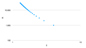
(b) Make a log-log graph of $R$ against $T$ in the resistance range from $1000\Omega$ to $30000\Omega$.

Relevant Equations

As far as I can tell (a) is super simple: just sub in the values of $R$, $a$, and $b$ and solve for $T$. I get the solution 0.56 when I do this (I am assuming this is in Kelvin).

The answer at the end of the book, however, is 4.01K.

As for (b), I understand this as simply subbing in the given values of $a$ and $b$ and solving for $T$ as a function of $R$.

I am not sure, however, what a log-log graph would be in this case

(a)

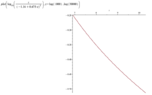
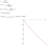
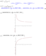
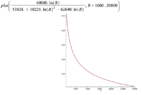
(b)

Here is a plot of this function T of R

It seems that as the resistance goes up the temperature goes down. Not sure what to make of this physically speaking.

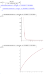
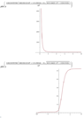
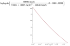
My question is about the requested log-log graph.

Above we have a function T of R, but we want a function $\log{T}$ of $\log{R}$.

Here is what I came up with

$$w=\ln{T} \implies T=e^w$$

$$z=\ln{R}$$

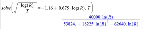
Then, since $T(R)=\frac{40000\ln{R}}{53824+18225(\ln{R})^2-62640\ln{R}}$ we have

$$e^w=\frac{40000z}{53824+18225z^2-62640z}$$

$$w=\ln{\left ( \frac{40000z}{53824+18225z^2-62640z} \right )}$$

We want to make a plot of $w$ as a function of $z$ in the range $z=\ln{1000}$ to $z=\ln{30000}$.

I am not sure why we were asked to make this particular graph. The first graph seems more interesting.

Does the reasoning and overall calculation steps make sense?

This problem is from the book "Heat and Thermodynamics" 7th Ed. by Zemansky and Dittman

 

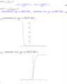
[BvU]

Homework Statement: The resistance $R$ of a particular carbon resistor obeys the equation

$\frac{\log{R}}{T}=a+b\log{R}$

Did you read what you posted ? Is there a square root missing ?

You use natural logarithm to get 0.56. What if you use base 10 (as some engineers happen to do sometimes ) ?

$\$

 

[Steve4Physics]

Just to add to what @BvU has said, the usual convention is:
'ln' is used for natural logarithms (base 'e').
'log' is used for logarithms base 10.
'
Logarithms to other bases are written explicitly, e.g. log₂(8) = 3.

 

[Merlin3189]

It seems that as the resistance goes up the temperature goes down. Not sure what to make of this physically speaking.

So how do you think you can change the resistance of " a particular carbon resistor " ?
(Hint: if it were a variable resistor -eg change the length of the carbon rod - then the relation you found would not hold. It is a particular piece of carbon, probably a thin film deposited on a ceramic substrate.)

You are better to see this as, "... as the temperature goes up the resistance goes down* ...", which is a concept familiar to you from high school science. (hints: Carbon. Lamp filaments. Ballast. Edison.)
(*Also, => vice versa)

 

[zenterix]

Did you read what you posted ? Is there a square root missing ?

You use natural logarithm to get 0.56. What if you use base 10 (as some engineers happen to do sometimes ) ?

$\$

Indeed there is a missing square root. The correct equation for the resistance of the carbon resistor is

$$\sqrt{\frac{\log{R}}{T}}=a+b\log{R}$$

Unfortunately, I can't edit the original question any longer.

 

[gmax137]

Indeed there is a missing square root. The correct equation for the resistance of the carbon resistor is
$$\sqrt{\frac{\log{R}}{T}}=a+b\log{R}$$

The answer at the end of the book, however, is 4.01K.

With the revised equation (including the square root) I get (at T=1000) R=4.01 as well.

 

[kuruman]

A general remark is that the statement of the problem should have specified that the numerical values for $a$ and $b$ assume that, in the formula, $R$ is in Ohms and $T$ Iis in Kelvin.

To @zenterix :
You were asked to make a log-log graph of $R$ against $T$ and you have produced two linear plots of $T$ against $R$. The convention is that you plot a dependent variable {against or vs. or as a function of} an independent variable.

To accomplish this, I suggest that you use a spreadsheet, which is most suitable for the task because it allows you to get the around having to solve the formula numerically.
1. Create a column of resistance values from 1000 Ω to 30,000 Ω.
2. Create a second column with the values for the right-hand-side of the formula (RHS).

At this point I don't want to give everything away so I will ask you, do you see how you can create a third column with the appropriate temperature values? If so, do it and plot. You will have to set the axes to "logarithmic" because the default value is "linear."

 

[zenterix]

Indeed you are all correct that I used the natural logarithm when I should have used the base 10 logarithm. Redoing the calculations shows this.

As for the loglog plot, analytically we have

Then, in Maple

Note that the values on the axes are of w and z. I am still figuring out how to actually get the scales in terms of T and R. The plot itself seems to be correct though and has the same shape as before: higher temperature, lower resistance.

 

[zenterix]

A general remark is that the statement of the problem should have specified that the numerical values for $a$ and $b$ assume that, in the formula, $R$ is in Ohms and $T$ Iis in Kelvin.

To @zenterix :
You were asked to make a log-log graph of $R$ against $T$ and you have produced two linear plots of $T$ against $R$. The convention is that you plot a dependent variable {against or vs. or as a function of} an independent variable.

To accomplish this, I suggest that you use a spreadsheet, which is most suitable for the task because it allows you to get the around having to solve the formula numerically.
1. Create a column of resistance values from 1000 Ω to 30,000 Ω.
2. Create a second column with the values for the right-hand-side of the formula (RHS).

At this point I don't want to give everything away so I will ask you, do you see how you can create a third column with the appropriate temperature values? If so, do it and plot. You will have to set the axes to "logarithmic" because the default value is "linear."

Indeed I should plot R as a function of T.

Let me see if I understand your spreadsheet suggestion (I'm going to interpret it without the last step of setting axes to logarithmic)

Create a column of R from 1000 to 30000.

Create a second column with the log of the first column, call this variable z.

Because we have the equation $T=\frac{\log{R}}{(a+b\log{R})^2}$, create a column that uses values from the second column: $\frac{z}{(a+bz)^2}$. This column represents T.

Create a fourth column of the log of the third column. This represents values $\log{T}$.

Now, plot the fourth column against the second column.

This won't give us the usual values of T and R with a logarithmic scale. It will simply be the logarithmic scale with the labels being the actual logs instead of the underlying variables we're taking the logs of. Still correct though.

If we solve the original equation analytically

Seems there are two solutions. If we plot them we get

Not clear which is the one we want.

 

[kuruman]

I don't know MAPLE and I cannot advise you on that but the plots you produced are not what you should be looking at. Yes, using $T=\dfrac{\log{R}}{(a+b\log{R})^2}$ is the way to get the temperature values. Once you have these, you can set up a columns of R values and a column of T values. Then get yourself a decent plotting program and follow one of the following plans.

Plan A
Plot R vs. T and set the axes on your plotting program to log-log. Log-log plots are useful to know how to do especially if you are looking for a power law linking the dependent to the independent variable.

Plan B
Create two more columns $y=\log_{10}(R)$ and $x=\log_{10}(T).$ Plot $y$ vs $x.$ The problem with Plan B is that the tick labels on the axes would be the logarithms of resistance and temperature and not the actual values. The shape of the curve would, of course, be the same.

 

[zenterix]

I don't know MAPLE and I cannot advise you on that but the plots you produced are not what you should be looking at. Yes, using $T=\dfrac{\log{R}}{(a+b\log{R})^2}$ is the way to get the temperature values. Once you have these, you can set up a columns of R values and a column of T values. Then get yourself a decent plotting program and follow one of the following plans.

Plan A
Plot R vs. T and set the axes on your plotting program to log-log. Log-log plots are useful to know how to do especially if you are looking for a power law linking the dependent to the independent variable.

Plan B
Create two more columns $y=\log_{10}(R)$ and $x=\log_{10}(T).$ Plot $y$ vs $x.$ The problem with Plan B is that the tick labels on the axes would be the logarithms of resistance and temperature and not the actual values. The shape of the curve would, of course, be the same.

It is not necessary to know Maple.

My goal is simply to present the equations and then use some software to plot. The crucial part are the equations.

Now, here is the spread sheet version you are talking about (Plan B):

First, the data

The first plot here is just R against T

Next we can plot the second column, log(R), against the last column, log(T)

Finally, we can take the first plot of R against T and simply tell the spreadsheet software to make the axes have a logarithmic scale (your Plan A)

This should be exactly the same as the second plot except that the labels on the axes are different because here we are showing R and T and previously we were showing their base 10 logs. The spacing here is based on the base 10 logs.

As for your comment on the plots I produced, I do believe that the first one matches the ones I showed from the spreadsheets. It's just that the spreadsheets are using a limited number of points. Let me illustrate again

If we solve the original equation for $\log_{10}{(R)}$ then we obtain

However, we want $\log_{10}{(R)}$ as a function of $\log_{10}{(T)}$, so we have

If we use new names for the logarithms, $w=\log_{10}{(R)}$ and $z=\log_{10}{(T)}$, then we have the equation

Which, after subbing in $a=-1.16$ and $b=0.675$, if we plot, should be the same plot as the second one from the spreadsheet (shown above).

Here is it

This matches the plot from the spreadsheet. The issue with this plot from my previous post is that the range I used for z was too large so the plot looked weird.

But it is in fact the same as the spreadsheet one.

Now, the question I still have is about the other solution when we solved for $\log_{10}{(R)}$.

I frequently have trouble with this type of question.

The problem stated that temperature and resistance obeyed a certain equation. When we solved that equation for $\log_{10}{(R)}$ we got a quadratic and two solutions.

I guess we just throw away the second solution, which generates the following plot

 

[zenterix]

So how do you think you can change the resistance of " a particular carbon resistor " ?
(Hint: if it were a variable resistor -eg change the length of the carbon rod - then the relation you found would not hold. It is a particular piece of carbon, probably a thin film deposited on a ceramic substrate.)

You are better to see this as, "... as the temperature goes up the resistance goes down* ...", which is a concept familiar to you from high school science. (hints: Carbon. Lamp filaments. Ballast. Edison.)
(*Also, => vice versa)

Indeed, it makes more sense to say "as the temperature goes up the resistance goes down".

 

[kuruman]

I think you have accomplished what you were asked to do. Here is the plot I made using plan A. It matches yours.