Magnetic Field Computation from Thick Rectangular Conductor

[MrManhattan]

Hello, and thanks in advance for taking a look at my question.

Generally, I am trying to make a railgun force model. Since railguns depend on the magnetic field created around the rails (and the resulting Lorentz force) I need to model the magnetic field created by the current that flows through the rails.

The problem is, when I compute the magnetic field using my implementation of Biot-Savart, I get something around 2500 T as an average field strength between 0 and 1.2 cm away from a 1 x 1 cm rail carrying 20,000 A of current (I get about 3100 T as a maximum closest to the rail). The magnetic field around a circular conductor (simplification made for a sanity check) is around 0.5 T closest to the "rail" when you take both rails into account. I cannot for the life of me figure out this huge discrepancy. I've checked units, I've quadruple-checked all my constants, I've run a mesh refinement analysis, I've even made an animation to show that my indexing is working properly. Perhaps most convincing is that when using another implementation of Biot-Savart (a more simple equation), I get a result pretty close to the simple wire value.
I have no idea what's wrong, and I'm hoping someone can help me out.

I should mention that I'm an aerospace engineering student, with a graduate focus in structures...so neither I, nor my advisor, are EM experts.

Here's a simple diagram if you're not familiar with railguns.

I am essentially using Biot-Savart to compute the magnetic field in a discrete armature section (P) from a discrete rail section (P'). I am doing this following equation 2 from this paper in MATLAB.

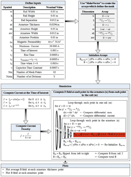
To my understanding, this equation shows the magnetic field at an arbitrary point (P: x,y,z) outside the rail. So, to find the magnetic field at each point in the armature, I currently use 5 loops. Two to loop through the rail positions (y' and z' with the long rail dimension being essentially infinite) and three to loop through the armature positions (x, y, z). I am following a test case Here is a block diagram of my current code.

Additional Question: Even though I'm not currently doing this, I will be adding a temporal loop as well. This will mean the length of rail producing magnetic field will change, and I will need to add a 6th loop to account for discrete rail sections in the x (long) direction. How do I define volumetric current density? The current is not contained in the long (flowing) direction that way. It seems incorrect to just divide current by the length of each section because the current flows that direction. However, I cannot just not divide because then my solution is simply a factor of my mesh size, since the magnetic field contribution from each section gets added together.

I am computing the integrals as simple sums (midpoint rule, I guess), but I see relatively little change by adjusting mesh size. If this sort of simple integration were a problem, I should see significant and unstable changes with mesh size, correct? Below is the mesh refinement analysis I did, where the average magnetic field is plotted for varying mesh size. As you can see, the one unstable variable is the mesh size of the armature width. As the size gets smaller, more elements get closer to the rail (r goes to 0) and this influences the average more than the other points in the center bring it down. But this doesn't show a problem with this formulation, correct?

Finally, here are links to my code. The input case I'm running is based off of this paper. That paper also contains the simplified version of Biot-Savart that seems to be working.

The more complicated Biot-Savart implementation I'm interested in fixing is the MATLAB code. The "Gif" section at the bottom (and option at the top) are only done to make a movie showing that point P' computes B field at point P, and then loops through all of these values. As I mentioned at the top, this was done to make sure my indexing runs correctly.
Gist || Dropbox

Required Function for the MATLAB Code:
Gist || Dropbox

The simpler Biot-Savart code is in the Mathematica code (Section ILR1). Everything in this code seems accurate with the exception of a mysterious factor of two in the ILR1 force integral, and the in-progress F1 section.
Gist || DropboxUpdate:

I have used MATLAB's integral2 to do the integration now. There are now only 3 loops in the computation. I loop through each armature position, and compute the magnetic field at that point by integrating over the rail sections. The old computation is in the code still for comparison.

The answer given by this code is different, but it still does not match up with the simpler wire code, or the simpler Biot-Savart equation. Instead of ~2500 T as an average, I get ~0.0025 T. And yes, most of the values are about a factor of 10^-6 different from the previous values. But, as I said, this doesn't match ~0.5 T that I get from the simpler formulations. Does anyone know why this might be ?

I still don't understand why I am getting such smaller values now. I know I was summing up each loop, but I was also dividing by the width and height, so I should get the same answer at the end. Especially since the result is stable with increasing mesh size...

Here is the code for the new file: Gist || Dropbox

For convenience, here is a hyperphysics calculator that does the wire calculation. To get the maximum value, I compute the B field at 0.01m (the width of the rail) and then add the B field at 0.01 + 0.012 m (the width of the second rail, plus the rail separation) to get ~0.5 T (this one actually comes out to ~0.58 T).

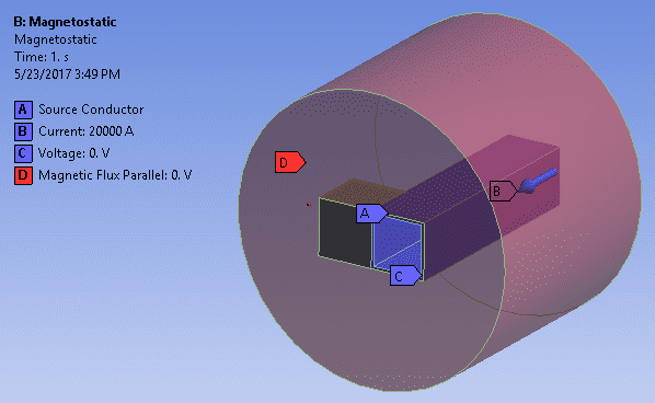
Additionally, I have run an ANSYS Workbench Magnetostatic simulation to check my values further. This gives me yet another result...

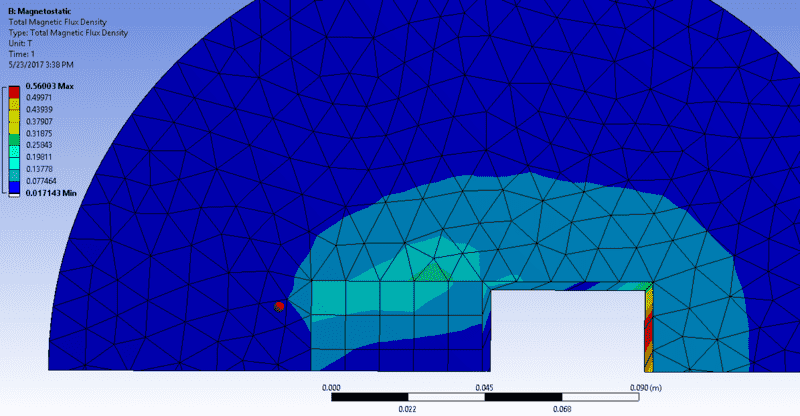
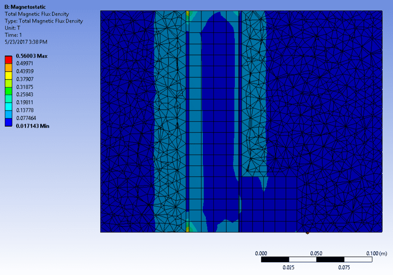
I made the mistake of using the wrong scale and going a little to detailed with this model, as you'll notice the rail is hollow (this is a way of getting around using a transient solution because in a railgun the current pulse is so fast, it operates like AC current and only travels in the skin of the rail...I'll deal with that in the rest of my analysis later). The reigon of square mesh next to the rail (copper) is the armature (aluminum), and the surrounding area is just air. I have run another version, but the simulation license is now being used by someone else, so I don't have that result to post. If I recall correctly, that result gave even smaller values. As you can see, the magnetic field in the armature is 0.017 to 0.19 T. Sure, this seems to be at least on the same order of magnitude, but, as shown by the second result image, most of the armature is near the low end of this. Yes, the other simulation has smaller values, but not something near what the MATLAB code is getting now (though I'd have trouble trusting that anyway since I believe the simple approximations the most). Would the result be significantly smaller because the Biot-Savart solutions don't consider the magnetic field needing to penetrate another metal?

 

[mfb]

10⁶ always sounds like a unit conversion issue.

Did you check how it scales with the relevant parameters? If you double the current, does the magnetic field double? If you reduce the width or height of the rail by a factor 2 (but keep current the same), does the magnetic field at the same position stay roughly the same?

How did you model the current flow at the armature/rail connection in ANSYS? I would expect that region to be quite challenging.

 

[MrManhattan]

10⁶ always sounds like a unit conversion issue.

Did you check how it scales with the relevant parameters? If you double the current, does the magnetic field double? If you reduce the width or height of the rail by a factor 2 (but keep current the same), does the magnetic field at the same position stay roughly the same?

How did you model the current flow at the armature/rail connection in ANSYS? I would expect that region to be quite challenging.

Yes, it does sound like a conversion issue, but the difference is between two models computed from the same constants. I can check to make sure there's no difference, but there shouldn't be. No, but I will check that tomorrow when I have more time with the license. I just have my memory to go off of at the moment, but I don't remember a significant change after changing the rail to a solid beam, and decreasing the rail from 5x5 cm to 1x1 cm.

Agreed. I'm not sure how I would do that with the workbench. I can do it with ANSYS Maxwell, but my laptop with that license is out of commission right now. Anyway, it's not an issue because the MATLAB and other codes don't consider the current flowing through the armature when computing the magnetic field ( the field generated by that current doesn't produce a significant force, so it's neglected ). So the ANSYS model just has the current flowing straight through the rail. The armature is just sitting there, like the surrounding air is.

 

[mfb]

Well, does the current suddenly stop at one x-coordinate? That is not what the actual current will do.

 

[MrManhattan]

Well, does the current suddenly stop at one x-coordinate? That is not what the actual current will do.

True. But in computing the armature force, there are two important quantities; the magnetic field that points in either the y or z directions ( up/down and left/right when the rails are pointing into the page ) and the current that flows through the armature. The magnetic field created by the current in the armature goes in a different direction, and so far as I'm aware, doesn't exist where the main current flows in the armature. Then, to compute the armature force, you just need to get the magnetic field created from the rails, and multiply it by the current flowing through the armature.

So I'm just trying to compute magnetic field from a thick rectangular conductor with the MATLAB code. The ANSYS stimulation I'm doing here is only validating those results, so it only needs to get magnetic field at some distance from the rail.

I will do an ANSYS Maxwell simulation that is more coherent and complete though.

 

[MrManhattan]

Okay, well I've mostly solved all of my issues. However, the idea that all is well hinges on a few assumptions that I'm not really comfortable with, and my results, while being on the same order of magnitude, are not particularly good compared to ANSYS.

When I compute "equation 2" in the "integral2" code, I was dividing by the height and width of the rail, like equaiton 2 prescribes. However, inside the integral, the field being computed comes from a current element with its own, much smaller, height and width. Changing the h and w to "dyp" and "dzp" (standing for dy' and dz') gives me an overall field maximum of ~0.46, which is relatively close to the ~0.51 from the more simple computations. So that's good news. The answer comes out to something somewhat reasonable.

But the discrepancy between using the integral function and pure summation remains at ~10^5. I am convinced, especially because of this latest discovery, that this is caused by an indexing error somewhere, but I am unable to find it. The very strange part, if it were an indexing error, is that the result is stable with changes in mesh size. Since using integral2 this deep into nested loops takes a very long time, and the solutions from the two methods are nearly identical (aside from this 10^5 factor), I have begrudgingly just divided the result of the summation by 10^5.

In staring at the more simple solutions more I have encountered an issue regarding that "mysterious factor of 2" I mentioned in the original post. I found this MIT paper that agrees with the equations in other papers, but not with the Hyperphysics equation I referenced before. The difference being a division by 4 (in the MIT reference and the two papers I referenced) and a division by 2 in the Hyperphysics equation. Now, generally I would just disregard the Hyperphysics equation as less reputable, and less specific than the other sources. But there's a twist. With the answers given from the simple equations, its easy to approximate railgun force, and compare it to this Waindok et. al. paper (that I linked before) and the "railgun force equation" (F = I^2 * L' / 2 , where L' is the inductance gradient of the rails and is usually ~ 0.5 * 10^ -6). If you took a look at the mathematica file, you would see that the railgun force equation gives a force of 97.946 N for this case, which is fairly close to the paper's "analytic ILR" force of 110 N. The Windok et. al. paper also mentions a force equation (equation 3 in that paper) that is easy to use, which gives a force of 97.7704 N. I'm a bit concerned because the paper's equation should give the paper's result exactly, not 10% off, but those are small fries compared to the issue I'm having now. When I compute railgun force using equation 2 from Waindok et. al. (the integral formulation), I get 48.8852 N. That's using the simple B field computation from that same paper. Similar results are obtained by using the MIT equation to find B. Notice that 48.8852 * 2 = 97.7704. There's an exact factor of two discrepancy between my implementation of equations 1 and 2 (integral formulation) and equation 3. So, if I use the Hyperphysics equation, I can get very close to the 97 N answer from the simple and Waindok et. al. force equations. Does anyone know the source of this factor of two difference?

A couple very useful pieces of information did come out of this whole debacle though. The equation 1 from Waindok et al. is just a different from of the finite wire equation from that MIT reference. Since, theta2 will always be 90 degrees, the MIT reference equation simplifies to B = mu0 * I / (4*pi*r) * cos( theta1 ) . Then, computing theta1 from the armature position (l) and the armature thickness gives theta1 = atan ( r / l ). We can then see that cos( atan ( r / l ) ) = l / sqrt( l^2 + r^2 ) as the Waindok et. al. equation uses. So, that tells me where that equation comes from. Further, and much more importantly, it solves the conundrum of discretizing current in its flow direction. I can't say I understand all the math behind it, but I now know that the length of the rail is accounted for in the equation 1 of Waindok et. al. and equation 2 of Lizhong et. al. (also from the original post).

Now, for the part with the pretty plots. I returned to ANSYS (though I didn't get a chance to compare changes in primary parameters) and looked at the case with similar geometry and scale. The results are somewhat similar, but I am getting a maximum B field of ~ 0.86 T (the maximum from one rail is 0.63 T, and the value at the far end is 0.23 T). Not a value of 0.46 or 0.51 like the other calculations got. I don't know how much of an effect the material properties have, so I'm really not sure what to make of this. If I account for material properties in my model, will I get a closer answer? I will try this tomorrow (along with changing the main parameters, and seeing how all the models change with respect to each other).

Anyway, here are the plots. The first, and most informative are of the armature rear face, then I show the whole armature, then the armature and rail, then the armature, rail, and surrounding air.

 

[mfb]

Does anyone know the source of this factor of two difference?

A typo in the paper? A different definition of L'?
You can write them a mail and ask them.

 

[MrManhattan]

A typo in the paper? A different definition of L'?
You can write them a mail and ask them.

Yeah, it could be the result of a typo, but doesn't only show up in the result from the Waindok et. al. paper. It also shows up in the "railgun force equation" and the equation on Hyperphysics (I'm not married to the site, but they've always had accurate information in the past, so far as I've seen). Not to mention the results that match fairly well with my result are repeated multiple times through the paper ("the results" being F_ILR = 110 N from the paper and my result being F = 97 N).

The L' definition is pretty standardized, here's a paper on it that has a good table (the S/H and W/H values are both 1.2 for this case). At the very least, L' shouldn't be a factor of 2 off of 0.5 uH.

Now, I'm much more convinced of a factor of 2 issue because ANSYS is coming up with a similar result. Even as I change scale and excitation current, I get a consistent factor of 2 increase from my more complex MATLAB result (which is agreeing fairly well with the more simple results) to the ANSYS result. Once I finish generating and processing the data today, I'll post it. But you can see this in the last results I posted. The maximum result I get from MATLAB is 0.4622 T. The maximum result from the ANSYS I posted is 0.63397 + 0.23861 = 0.8726. I should say that the ANSYS result I'm getting now is slightly higher at 0.9096.

Hopefully I don't come off too defensive / argumentative, since I'm just telling you repeatedly that I don't think the thing you suggested is my problem. I very much appreciate you taking a look at this, and offering ideas.

 

[MrManhattan]

Attached are some plots that show the ANSYS vs. MATLAB results. But more importantly, I've noticed an issue with the shape of the MATLAB results. When plotting these, I plot the magnetic field as a 3D surface where X is the width of the armature, Y is the height of the armature, and Z is the magnetic field strength. Then I plot surfaces for the different armature thickness values (x direction from the paper described earlier, the long direction of the rails) as separate surfaces. As expected, the "deeper" (further away from the armature rear face) into the armature I go, the lower the magnetic field. For the first (top in the plot, on the rear face physically) surface, the shape makes sense. There is a decrease in the center, as this is farther from each rail, and there is a decrease at the top and bottom. This is reasonable because, say, the top of the armature is furthest away from the current flowing through the bottom of the rail. The middle of the armature is closer to both the top and bottom, and should thus have a higher magnetic field. However, the subsequent surfaces have a different shape, and do not fall off in the center of the armature. I thought it possible that there was some adjustment made to the equation I'm using to account for current through the armature (as you were mentioning earlier). But this equation is only for By (B field in the y direction used in the Lizhong et. al. paper), and that current would create no B field in that direction. I cannot figure out the reason for this shape difference, and though the value along the rear face is most important, I'd like to have a computation that actually works. Here is the plot I was talking about showing 5 armature thickness surfaces.

When scaling the model up and down a little bit (0.5x and 2x) I get an inverse linear change in results (all geometric values / 2 gives magnetic field strength increases by 2x). This gives results that are fairly close to twice as large as the MATLAB result (corresponding to the factor of 2 that I have been talking about). The maximum values, and the majority of the overall values seem to follow this trend, but the minimum values do have a bit smaller than 50% error. So it's possible that I'm just looking for a factor of 2 and just seeing it everywhere.

However, when I change the scale to 0.1x or 10x, I get very strange results (which is why these results are left out of the MATLAB plots). Both results have shapes that do not seem reasonable. First, the 0.1x scale plot shows a ball of very high magnetic field in the middle of the armature...I cannot explain this. I'm somewhat willing to ignore it though, since a 0.1x scale would be a 1x1 mm rail, which would never be used in practice. The first plot shows a slice halfway through the height of the armature and rail. The second plot shows a slice through just the armature, which really shows this "swirling" B field. The last plot is the rear fact of the armature, corresponding to an image from earlier, the 10x scale figure below, and the MATLAB plot below that.

The 10x scale simulation also shows a seemingly incorrect shape, as there is a magnetic field concentration near the top and bottom of the armature. This doesn't make sense as it conflicts with the rationale I described for liking the MATLAB plot above.

Here is a plot from MATLAB showing the magnetic field strength over this rear armature face for just two thickness values (which I think is easier to look at). If this is compared to the results from my earlier post, it matches up well (the ANSYS result only has one rail, so that explains the lack U shape in the armature width direction). This shape is also followed by the 0.5x and 2x scale cases, as well as the changing current cases.

 

[MrManhattan]

...forgot to include the ANSYS vs. MATLAB comparison plots