- #1
DrWahoo
- 53
- 0
This is the code for Sensitivity Analysis via Rosenwasser's method. Code was for my Masters Thesis, so maybe it will be useful to someone in Dynamical Systems or Modeling with ODE's
View attachment 7549
View attachment 7550
View attachment 7551
View attachment 7552
Code:
function ode45_both_age
%--------------------------------------------------------------------------
% Solves the sensitivity equations for the age structure omnivory model.
%
% Input: None
%
% Output: Graphs of norms of sensitivities over time.
%--------------------------------------------------------------------------
close all
%--------------------------------------------------------------------------
% Define "Input" Parameters
%--------------------------------------------------------------------------
tn = 1600; % ending time
y0 = [1; 1; 1 ; 2; 0; 0; 0; 0]; % initial values
w_P1 = 2; % weight on the adult predator sensitivity for the norm
w_P2 = 2; % weight on the juvenile predator sensitivity for the norm
w_C = 2; % weight on the consumer sensitivity for the norm
w_R = 2; % weight on the resource sensitivity for the norm
norm_s = zeros(2100,15); % initialize a matrix to hold the norms of
% sensivities (columns) at each time step
% (rows).
parameter = 1; % = 1, then use parameter values from literature
% otherwise use my favorite parameter values
%---Parameters to be passed to rhs_both
if parameter == 1
eRP = 0.4;
eCP = 0.69;
eRC = 0.7;
aRP = 0.045;
aCP = 0.025;
aRC = 0.025;
hRP = 4;
hCP = 4;
hRC = 3;
mP = 0.03;
mJ = 0.04;
mC = 0.027;
nP = 0.06;
r = 0.3;
K = 4;
else
eRP = .3;
eCP = 0.43;
eRC = 0.6;
aRP = 0.0275;
aCP = 0.025;
aRC = 0.04;
hRP = 4;
hCP = 5;
hRC = 3;
mP = 0.06;
mJ = 0.1;
mC = 0.11;
nP = 0.1;
r = 0.3;
K = 8;
end
%--------------------------------------------------------------------------
% Solve the state and sensitivity systems simultaniously
% y = column vector (length 8) of states and sensitivities
% y(1) = adult predator density,
% y(2) = juvenile predator density
% y(3) = consumer density,
% y(4) = resource density,
% y(5) = adult predator sensitivity,
% y(6) = juvenile predator sensitivity
% y(7) = consumer sensitivity
% y(8) = consumer sensitivity
%--------------------------------------------------------------------------
% eRP
p = 1;
[t_1,y] = ode45('rhs_both_age',tn,y0,[],p,eRP,eCP,eRC,aRP,aCP,aRC,hRP,hCP,hRC,mP,mC,nP,r,K,mJ);
L_1 = length(t_1);
norm_s(1:L_1,p) = sqrt(w_P1.*(y(:,5)).^2 + w_P2.*(y(:,6)).^2 + w_C.*(y(:,7)).^2 + w_R.*(y(:,8)).^2);
% eCP
p = 2;
[t_2,y] = ode45('rhs_both_age',tn,y0,[],p,eRP,eCP,eRC,aRP,aCP,aRC,hRP,hCP,hRC,mP,mC,nP,r,K,mJ);
L_2 = length(t_2);
norm_s(1:L_2,p) = sqrt(w_P1.*(y(:,5)).^2 + w_P2.*(y(:,6)).^2 + w_C.*(y(:,7)).^2 + w_R.*(y(:,8)).^2);
% eRC
p = 3;
[t_3,y] = ode45('rhs_both_age',tn,y0,[],p,eRP,eCP,eRC,aRP,aCP,aRC,hRP,hCP,hRC,mP,mC,nP,r,K,mJ);
L_3 = length(t_3);
norm_s(1:L_3,p) = sqrt(w_P1.*(y(:,5)).^2 + w_P2.*(y(:,6)).^2 + w_C.*(y(:,7)).^2 + w_R.*(y(:,8)).^2);
% aRP
p = 4;
[t_4,y] = ode45('rhs_both_age',tn,y0,[],p,eRP,eCP,eRC,aRP,aCP,aRC,hRP,hCP,hRC,mP,mC,nP,r,K,mJ);
L_4 = length(t_4);
norm_s(1:L_4,p) = sqrt(w_P1.*(y(:,5)).^2 + w_P2.*(y(:,6)).^2 + w_C.*(y(:,7)).^2 + w_R.*(y(:,8)).^2);
% aCP
p = 5;
[t_5,y] = ode45('rhs_both_age',tn,y0,[],p,eRP,eCP,eRC,aRP,aCP,aRC,hRP,hCP,hRC,mP,mC,nP,r,K,mJ);
L_5 = length(t_5);
norm_s(1:L_5,p) = sqrt(w_P1.*(y(:,5)).^2 + w_P2.*(y(:,6)).^2 + w_C.*(y(:,7)).^2 + w_R.*(y(:,8)).^2);
% aRC
p = 6;
[t_6,y] = ode45('rhs_both_age',tn,y0,[],p,eRP,eCP,eRC,aRP,aCP,aRC,hRP,hCP,hRC,mP,mC,nP,r,K,mJ);
L_6 = length(t_6);
norm_s(1:L_6,p) = sqrt(w_P1.*(y(:,5)).^2 + w_P2.*(y(:,6)).^2 + w_C.*(y(:,7)).^2 + w_R.*(y(:,8)).^2);
% hRP
p = 7;
[t_7,y] = ode45('rhs_both_age',tn,y0,[],p,eRP,eCP,eRC,aRP,aCP,aRC,hRP,hCP,hRC,mP,mC,nP,r,K,mJ);
L_7 = length(t_7);
norm_s(1:L_7,p) = sqrt(w_P1.*(y(:,5)).^2 + w_P2.*(y(:,6)).^2 + w_C.*(y(:,7)).^2 + w_R.*(y(:,8)).^2);
% hCP
p = 8;
[t_8,y] = ode45('rhs_both_age',tn,y0,[],p,eRP,eCP,eRC,aRP,aCP,aRC,hRP,hCP,hRC,mP,mC,nP,r,K,mJ);
L_8 = length(t_8);
norm_s(1:L_8,p) = sqrt(w_P1.*(y(:,5)).^2 + w_P2.*(y(:,6)).^2 + w_C.*(y(:,7)).^2 + w_R.*(y(:,8)).^2);
% hRC
p = 9;
[t_9,y] = ode45('rhs_both_age',tn,y0,[],p,eRP,eCP,eRC,aRP,aCP,aRC,hRP,hCP,hRC,mP,mC,nP,r,K,mJ);
L_9 = length(t_9);
norm_s(1:L_9,p) = sqrt(w_P1.*(y(:,5)).^2 + w_P2.*(y(:,6)).^2 + w_C.*(y(:,7)).^2 + w_R.*(y(:,8)).^2);
% mPA
p = 10;
[t_10,y] = ode45('rhs_both_age',tn,y0,[],p,eRP,eCP,eRC,aRP,aCP,aRC,hRP,hCP,hRC,mP,mC,nP,r,K,mJ);
L_10 = length(t_10);
norm_s(1:L_10,p) = sqrt(w_P1.*(y(:,5)).^2 + w_P2.*(y(:,6)).^2 + w_C.*(y(:,7)).^2 + w_R.*(y(:,8)).^2);
% mC
p = 11;
[t_11,y] = ode45('rhs_both_age',tn,y0,[],p,eRP,eCP,eRC,aRP,aCP,aRC,hRP,hCP,hRC,mP,mC,nP,r,K,mJ);
L_11 = length(t_11);
norm_s(1:L_11,p) = sqrt(w_P1.*(y(:,5)).^2 + w_P2.*(y(:,6)).^2 + w_C.*(y(:,7)).^2 + w_R.*(y(:,8)).^2);
% nP
p = 12;
[t_12,y] = ode45('rhs_both_age',tn,y0,[],p,eRP,eCP,eRC,aRP,aCP,aRC,hRP,hCP,hRC,mP,mC,nP,r,K,mJ);
L_12 = length(t_12);
norm_s(1:L_12,p) = sqrt(w_P1.*(y(:,5)).^2 + w_P2.*(y(:,6)).^2 + w_C.*(y(:,7)).^2 + w_R.*(y(:,8)).^2);
% r
p = 13;
[t_13,y] = ode45('rhs_both_age',tn,y0,[],p,eRP,eCP,eRC,aRP,aCP,aRC,hRP,hCP,hRC,mP,mC,nP,r,K,mJ);
L_13 = length(t_13);
norm_s(1:L_13,p) = sqrt(w_P1.*(y(:,5)).^2 + w_P2.*(y(:,6)).^2 + w_C.*(y(:,7)).^2 + w_R.*(y(:,8)).^2);
% K
p = 14;
[t_14,y] = ode45('rhs_both_age',tn,y0,[],p,eRP,eCP,eRC,aRP,aCP,aRC,hRP,hCP,hRC,mP,mC,nP,r,K,mJ);
L_14 = length(t_14);
norm_s(1:L_14,p) = sqrt(w_P1.*(y(:,5)).^2 + w_P2.*(y(:,6)).^2 + w_C.*(y(:,7)).^2 + w_R.*(y(:,8)).^2);
% mPJ
p = 15;
[t_15,y] = ode45('rhs_both_age',tn,y0,[],p,eRP,eCP,eRC,aRP,aCP,aRC,hRP,hCP,hRC,mP,mC,nP,r,K,mJ);
L_15 = length(t_15);
norm_s(1:L_15,p) = sqrt(w_P1.*(y(:,5)).^2 + w_P2.*(y(:,6)).^2 + w_C.*(y(:,7)).^2 + w_R.*(y(:,8)).^2);
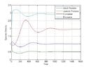
x = y(:,1:4); % State variables
%---Plot the states versus time
figure(7)
plot(t_15,x)
grid;
ylabel('Species Density');
xlabel('Time');
legend('Adult Predator','Juvenile Predator','Consumer','Resource') %---Plot the norms versus time
figure(100)
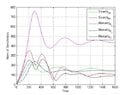
plot(t_7,norm_s(1:L_7,7),'b') %hRP
hold on
plot(t_8,norm_s(1:L_8,8),'g') %hCP
hold on
plot(t_9,norm_s(1:L_9,9),'r') %hRC
hold on
plot(t_14,norm_s(1:L_14,14),'k') % K
grid;
ylabel('Norm of Sensitivities');
xlabel('Time');
legend('Handling_{RP}','Handling_{CP}','Handling_{RC}','K') figure(200)
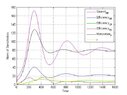
plot(t_4,norm_s(1:L_4,4),'m') %aRP
hold on
plot(t_1,norm_s(1:L_1,1),'b') %eRP
hold on
plot(t_2,norm_s(1:L_2,2),'g') %eCP
hold on
plot(t_3,norm_s(1:L_3,3),'r') %eRC
hold on
plot(t_12,norm_s(1:L_12,12),'k') %nP
hold on
plot(t_13,norm_s(1:L_13,13),'y') %r
grid;
ylabel('Norm of Sensitivities');
xlabel('Time');
legend('Search_{RP}','Efficiency_{RP}','Efficiency_{CP}','Efficiency_{RC}','Maturation_{P}','r')
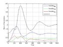
figure(300)
plot(t_5,norm_s(1:L_5,5),'g') %aCP
hold on
plot(t_6,norm_s(1:L_6,6),'r') %aRC
hold on
plot(t_10,norm_s(1:L_10,10),'m') %mPA
hold on
plot(t_15,norm_s(1:L_15,15),'b') %mPJ
hold on
plot(t_11,norm_s(1:L_11,11),'k') %mCgrid;
ylabel('Norm of Sensitivities');
xlabel('Time');
legend('Search_{CP}','Search_{RC}','Mortality_{P_{2}}','Mortality_{P_{1}}','Mortality_{C}')View attachment 7549
View attachment 7550
View attachment 7551
View attachment 7552