Runge-Kutta 4 w/ some sugar on the top: How to do error approximation?

[bremenfallturm]

TL;DR Summary

I know that the absolute error (for Runge-Kutta 4, and many other methods) is defined as $\text{values at step length } h - \text{values at step length } 2h$ (Def. 1). For my numerical approach to solving the problem, I don't get $\text{length } \text{values at step length } h = \text{length } \text{values at step length } 2h \cdot 2$ (Eqn. 1), which I think this has to do with the fact that I'm changing the step length near zero crossings. I need help finding out how to calculate the error

Hello! I'm currently working with a problem which allows modelling ball motion
$$\begin{aligned} m \ddot{x} & =-k_x \dot{x} \sqrt{\dot{x}^2+\dot{y}^2} \\ m \ddot{y} & =-k_y \dot{y} \sqrt{\dot{x}^2+\dot{y}^2}-m g \end{aligned}$$
Given that $k_x, k_y=0.005$, $m=0.01$ and $g=9.81$ and when $y$ crosses zero, $\dot y$ should change sign.
The initial conditions are $y(-1.2)=0.3$, $\dot y(-1.2)=0$, $\dot x(-1.2)=4$

I stated the equation above for context, but I don't think that it is the core of my question.

More about the problem:

• The differential equation is related to a ball moving on a plane surface, starting in $x=-1.2$ and ending in $x=1.2$. The latter is my stop condition (see below).
• The question is to find out the value of $y$ at any given point $x_0$ with an error smaller than $\mathcal O$.

I'm new to this forum and have used Matlab to solve the problem, but it seems to me like the Matlab category is more for the coding aspect of things. This question is more algorithm-oriented and specifically about error approximation. I apologize if I put it in the wrong place.

My current algorithm to solve this differential equation is:
I will refer to "Runge-Kutta 4" as RK4 below.

1. I have rewritten the system as a set of first order ODE:s. I will denote that $\vec u$.
2. Using Runge-Kutta 4 with a step length $h$, run until $y<0$. When that happens, go back to the $n-1$th iteration, and run RK4 with a finer step length. The step length is divided by two until $y_{\text{zero crossing}} < \mathcal O$ and $|x_{\text{zero crossing}}(h)-x_{\text{zero crossing}}(2h)| < \mathcal O$, where $\mathcal O$ is the error tolerance. This allows me to more precisely calculate the zero crossings. Running with a fine step length over the whole interval takes many minutes to complete, whilst this approach takes a couple of seconds.
3. When we know the zero crossing precisely, store the $\vec u$ values that were calculated in (3) with the fine step length. Flip the sign of $\dot y$ of $\vec u_{\text{zero crossing}}$. Finally, recalculate with RK4 the value for $\vec u_{\text{zero crossing}}$ with the flipped velocity.
4. Continue until $x>=1.2$

What I then do to finalize the problem (see "More about the problem" above):
5. To find the value of $x=x_0$, pick the $n+1$ $x$-values around $x_0$ and interpolate. I calculate the error by using
$|P_{n+1}-P_{n}(x_0)|$, where $P_n$ gives the $y$-value of the interpolated polynomial with degree $n$ at $x_0$.
Here, also given the conditional that $|P_{n+1}-P_{n}(x_0)|<\mathcal O$

______
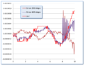
The solution is plotted below

The thing I'm having problems with is the error calculation of the main RK4 process. From above I know that:
$$\begin{cases}
E_{k\text{:th zero crossing}} = |x_{\text{zero crossing}}(h)-x_{\text{zero crossing}}(2h)| \\
E_{\text{interpolation}} = |P_{n+1}-P_{n}(x_0)|
\end{cases}$$
I have, however, used RK4 for the whole calculations, just not the zero crossings.
TL:DR this is my statement of the problem:
My problem is that I know that the absolute error (for Runge-Kutta 4, and many other methods) is defined as $\text{values at step length } h - \text{values at step length } 2h$ (Def. 1). When I try to run my code with step size $h$, I don't get the length of $\text{length } \text{values at step length } h = \text{length } \text{values at step length } 2h \cdot 2$ (Eqn. 1). I think this has to do with the fact that I'm changing the step length near zero crossings (see 2. in my algorithm).

Hence, the question: how should I figure out the error for the main Runge-Kutta 4 iterations in this case?
The problem is that vectors do not line up in size, and even if Eqn. 1 would be true, it feels kind of funky to take "every second element of the vector with the finer step length" subtracted with the previous iteration to calculate the error.
I have learnt about Richardson's extrapolation and thought that it might be viable here. But what should I Richardson extrapolate? Every value calculated with Runge-Kutta 4? The points included at the interpolation near $x = x_0$?

I hope I've outlined my problem and approach clearly enough and that it can be understood.
If not, please let me know what's missing! (Let's hope I didn't forget anything critical, heh)

 

[BvU]

TL;DR Summary: I know that the absolute error (for Runge-Kutta 4, and many other methods) is defined as $\text{values at step length } h - \text{values at step length } 2h$ (Def. 1).

Hello and !

I don't know that. What I seem to remember is that a truncation error estimate can be found from $y(x+h)- y(x+h/2+h/2)$ ($(7.17)$ here ).

For my numerical approach to solving the problem, I don't get $\text{length } \text{values at step length } h = \text{length } \text{values at step length } 2h \cdot 2$ (Eqn. 1), which I think this has to do with the fact that I'm changing the step length near zero crossings. I need help finding out how to calculate the error

I don't follow: what do you mean 'you don't get' $$\text{length } \text{values at step length } h = \text{length } \text{values at step length } 2h \cdot 2 \ ?$$ (I assume $2h\cdot 2$ is a mistake and you mean $(h/2)\cdot 2$ ?
In that case what you are saying is $y(x+h) \ne y(x+h/2+h/2)$ which is precisely the idea !

...

• The question is to find out the value of $y$ at any given point $x_0$ with an error smaller than $\mathcal O$.

My interpretation: you want to find the $x$ coordinates of the points where $y=0$ with an accuracy of $\mathcal O$. Right ?
Or do you want the absolute (accumulated!) error for all $y$ to be $\le \mathcal O$ ? (because that is what you appear to be saying!)

1. I have rewritten the system as a set of first order ODE:s. I will denote that $\vec u$.

To be explicit: $\vec u =(x,\dot x,y,\dot y)$ and 'the system' is $\dot{\vec u} = \vec f(\vec u)$. Right ?

2. Using Runge-Kutta 4 with a step length $h$, run until $y_{\bf\color{red}n}<0$. When that happens, go back to the $n-1$th iteration, and run RK4 with a finer step length.

The step length is divided by two to $h/2^i$ until ${\color{red}|}y_i{\color{red}|}< \mathcal O$ and $h/2^i - h/2^{i+1} < \mathcal O$, where $\mathcal O$ is the error tolerance.

Sorry to be so exact but we really need to be on the same page as the computer ...

I'm posting what I have so far; please check and correct where needed ...

$\$

 

[bremenfallturm]

Hello and thank you for your input. Let's first clarify what wasn't clear!
First off, "the system" is defined the way you put it in your post.
Same for the condition to find the zero crossing (step 2 in my algorithm, the last thing you quoted and clarified), you defined it better and that's also what I'm doing in my code

I don't know that

Hmm, that's how we have calculated the truncation error in the numerical analysis course I'm taking. Unfortunately the lecture material is not in English.
Does it help showing you this part of the lecture slides? I believe math is quite a universal language, if I can fill in the details.
This example from my teacher finds $y(0.2)$ with $y'=1+x-y$, given $y(0)=1$
First with $x_0=0$ and with step length $h=0.2$

Then with the step size $0.1$ ($h/2$)

Finally she concludes that the truncation error is $|y_{\text{at }x=0.2}(2h)-y_{\text{at }x=0.2}(h)$

(Sadly this is the best I can show you to prove my point)

I don't follow: what do you mean 'you don't get'

When I run my Runge-Kutta 4 over the whole interval, i.e. from $x=-1.2$ to when $x\geq 1.2$, including the process where I use a more fine step length near zero, I would expect (at least ideally) to get twice as many points for $y$ in my solution vector if I make the step length twice as big.
That is not the case, if I calculate over the whole interval.

I assume this is related to the fact that I use a finer step length with a "open/loose" conditional (run until the error is less than). If I skip the finer step length part, and just check the behavior of my solutions for y before the finer step length kicks in for the first time, I indeed get the relation that
the number of solutions increases by a factor two when the step length does so too.

This is trivial I guess, but the point I'm trying to make is that it makes comparing the solution vectors as different step length difficult because I'm using a finer step length near zero.

My interpretation: you want to find the x coordinates of the points where y=0 with an accuracy of O. Right ?

Not really. What I want to is find the value of $y$ at a given point $x_0$ with an accuracy of $\mathcal O$. But that's all I need!

I've always thought I need to check the whole error accumulation on the vector, but I realize that's not the case when I quote what my lecturer did. This pretty much makes a lot of my question useless, as I'm asking about how I should handle error calculation when I can't subtract the vectors $\text{all solutions at step length } 2h - \text{all solutions at step length } h$ using some simple kind of manipulation.

The solution to how to calculate the error of the main RK4 with step length $h$, might just be to find the $y_{\approx x_0}$ aka the $y$ that is closest to $x_0$, and given a step size of $h$, calculate
$y_{\approx x_0}(2h)-y_{\approx x_0}(h)$?

Sorry if things are still unclear, let me know what's missing if so. I do not mind explaining further.

 

[BvU]

this is the best I can show you to prove my point

We are talking about the same thing. Bear in mind that it's an estimate (See MIT 7.17)

The difference between a single step and two half-steps provides an estimate of the local error in the step. Such an error estimate...

Same for the condition to find the zero crossing (step 2 in my algorithm, the last thing you quoted and clarified), you defined it better and that's also what I'm doing in my code

Can we examine the code ? I'm struggling to follow your $$
\begin{cases}

E_{k\text{:th zero crossing}} = |x_{\text{zero crossing}}(h)-x_{\text{zero crossing}}(2h)| \\

E_{\text{interpolation}} = |P_{n+1}-P_{n}(x_0)|

\end{cases}$$doesn't it mean you always end up at a fixed number of halving the steps until $h_i - h_{i-1} <\mathcal O$ ? Or is $|\Delta y| < \mathcal O$ always the last condition met ?

$\$

 

[bremenfallturm]

Can we examine the code ? I'm struggling to follow your

Actually no, so sorry. This is an assignment for a course I am attending, with the explicit statement that "It is allowed to discuss the problem with others, but please don't share any code!"

doesn't it mean you always end up at a fixed number of halving the steps until hi−hi−1<O ? Or is |Δy|<O always the last condition met ?

Taking a quick check at my code, Scratch that, I actually had to analyze my results a little. Now I think I know what happens!
It looks like the error $h_i-h{i-1}<\mathcal O$ is the limiting factor when solving using the provided value of the initial velocity and $h=5\cdot 10^{-4}$ for the first two bounces (see the image I posted earlier). However, at the last bounce at the same step length, aka. the third and final bounce $|\Delta y| < \mathcal O$ (Cond. 2) becomes the limiting factor.

Does that make sense?

 

[BvU]

Actually no, so sorry. This is an assignment for a course I am attending, with the explicit statement that "It is allowed to discuss the problem with others, but please don't share any code!"

Ok, but I'm not handing in your work if that's what needs to be avoided

A bit hard to make quantitative remarks without code...

Taking a quick check at my code, Scratch that, I actually had to analyze my results a little. Now I think I know what happens!
It looks like the error $h_i-h_{i-1}<\mathcal O$ is the limiting factor ...

Seems to be rather a waste of CPU time to calculate all those derivatives when you know where it will stop...

when solving using the provided value of the initial velocity and $h=5\cdot 10^{-4}$ for the first two bounces (see the image I posted earlier).

So you start with step size 0.0005 ?
And what do you use for $\mathcal O$ ?

Using Runge-Kutta 4 with a step length h, run until y<0.

Seems a bit wasteful too: if $y<0$ occurs at step $n$ then at step $n-1$ a check of $y+h\dot y$ may already be enough to begin reducing step size !

And, RK4 evaluates the derivative at four points, so plenty of opportunities to see $y<0$ coming up !

 

[BvU]

Further comments:
The error estimate is for the local error. For the global error you have to factor in the number of steps.
I still wonder about your algorithm to locate $y=0$ points -- in connection with the notion that your real concern is the global error.
I wonder if it isn't equally accurate to take a single step of size $y_{n-1}/|\dot y_{n-1}|$ instead of $h$ if a step size $h$ causes $y_n < 0$.
It certainly would be a lot more efficient !

Lack of code made me do Good old Euler

Step size 0.01
Tedious but fun. Would be nice to compare the $x$ where $y=0$




$\$

 

[BvU]

Coming back to that global error. Here is an RK4.F90 including a simple test: $\ddot y = -y, \ y(0)=1, \dot y = 0$ from x=0 to 10. The answer is a cosine. Ran it with 50 steps, 100, 200, 400. Error $\equiv y(x)-\cos(x)$ plotted. Clearly 50 and 100 steps is not good enough (although all within $10^{-4}$ ).

200 and 400 steps are more interesting. Some up and down and disruption after x=8. Bright red line is $u-v$, i.e. $y(+h)-y(+h/2+h/2)$ , the local truncation error estimate.
As you can see, a lot is going on. And a lot can go wrong -- which Murphy states it will.

Disclaimer: I hope Excel cosine calculation is not the culprit. Burkardt f90 seems ok (but I have to jump 45 years from my fortrran IV and VAX fortran to nowadays fancy IDE so ).

[edit] Spikes are artefact: turns out a few variables were real instead of real*8 (double precision). Fixed, and all error plots are completely smooth. And $u-v$ is about 94% of the error.[edit 2] have to withdraw this. $u-v$ does not follow from comparing two runs with e.g. 4000 and 8000 steps

Blue and red lines in plot below are all right. Green line compares $y$ from 4000 steps with corresponding (but not exacly equal) $y$ from 8000 steps. Since latter are 2⁴ times closer to the cosine, green line is 15/16 of red line.

Sorry for the distraction.

$\$

 

[bremenfallturm]

Hello! Let me begin with a big thanks for all the help so far! This is my first numerical analysis course and as a first-year university student, your help and input is invaluable!

Ok, but I'm not handing in your work if that's what needs to be avoided

A bit hard to make quantitative remarks without code...

I understand that. Policies are policies, I guess - the assignment description encourages discussing the problems with others but is very clear that no code should be shared. I will of course abide by those rules and I understand it will limit your ability to help.

Seems to be rather a waste of CPU time to calculate all those derivatives when you know where it will stop...

Is it possible you could elaborate a little more on this point? I'm struggling a bit to follow along a bit with what you mean with "when you know it will stop".

So you start with step size 0.0005 ?
And what do you use for O ?

I've now changed it to $0.000\mathbf05$. $\mathcal O$ is $0.5\cdot 10^{-6}$, which is the highest error tolerated by the assignment.

Seems a bit wasteful too: if y<0 occurs at step n then at step n−1 a check of y+hy˙ may already be enough to begin reducing step size !

Ah yes, I see what you mean. Wouldn't implementing this change save me just a few iterations though? Given that the $x$-interval is so limited and that the number of bounces also is. I'm thinking this would be the case since Runge-Kutta 4 calculates the derivative in 4 points, so I would maximum save 4 iterations per bounce.

Lack of code made me do Good old Euler

Haha, nice! You asked for x-values for comparison for fun, here's what I get using the initial conditions given in the top post: (for the three bounces before $x=1.2$)

-3.53496e-01 4.3385e-01 9.1342e-01

I still wonder about your algorithm to locate y=0 points -- in connection with the notion that your real concern is the global error.

I've been pondering about that too, yes. I agree with you that it feels a little like fishing: throwing out a line, hoping for the best, and then repeating until you catch something.

I now have values for everything that the assignment asks for, but I will admit I am not completely satisfied with the algorithm. The problem is I am, as you might notice, still missing some puzzle pieces to figure out a better alternative.

Footnote:
I also have a follow-up question about how to approximate the error using a method whose English name I do not know. I am unsure whether to start a new topic or not, it's a footnote and I'd rather be sure about the method I'm using to calculate zero crossings but it's something I also need to figure out.

I hope you don't mind I briefly state what the question is about, I'm still new here and need to figure out if it's a good idea to start a new topic or not.

To directly translate this method from what we call it in my language would be "distrubance counting". I've been trying to find the English name for months, haha!
The principle is. Let's say you have a function $f(x,y,z)$ where $x, y, z$ have insecurities $\pm 1%$ as an example What you do is, try each combination: $f(x\cdot 1.01, y, z)$, $f(x, y\cdot 1.01, z)$, ...,
$f(x\cdot 0.99, y, z)$, ..., $f(x\cdot 1.01, y\cdot 1.01, z)$, and so on.
If you compare the differences from $f(x,y,z)$ for each value, an estimate of the global error is
$$
\sum \left|\Delta \right|
$$
The given values that have insecurities are $m$, $k_x$ and $k_y$. I have multiple numerical methods in my code: Runge-Kutta 4, interpolation, bisection method (used for a later part of the code, where the velocity is unknown but instead that $x(0)=0.3$). I'm wondering if the meaning of this method is that I should simply watch how the output for all the combinations change with all those combinations disturbed at the input level, or if I also need to fiddle around with disturbing outputs internally (disturbing the output of the interpolation before moving on to the bisection method for example). To me that doesn't really seem like what I should do, but discussing the problem with some others suggested that I might need to do that.

Is that a question different/big enough for a new topic?

 

[BvU]

$\qquad$ !​

This is my first numerical analysis course

Great ! I didn't have any formal NA courses but picked up quite a bit while going along.

the assignment description ... which is the highest error tolerated by the assignment ...

That assignment itself probably isn't a secret. Cold you post the full text verbatim ? What is fixed (given), what is required, what is optional, etc.

Is it possible you could elaborate a little more on this point?
...
Ah yes, I see what you mean

Well, with a step size of 5e-5 and an $\mathcal O$ of 5e-7 it takes about seven times of halving the step size before $h<\mathcal O$. Close to 30 'function evaluations'. As you said:

It looks like the error $h_i-h_{i-1}<\mathcal O$ is the limiting factor ...

And I'm not convinced that such an approach yields a much more accurate determination of the value of $x$ for which $y=0$.

-3.53496e-01 4.3385e-01 9.1342e-01

-0.338 0.466 0.965 I surely lose that with Euler and 0.01 steps. No wonder. Once I get RK4 going I'll come forward again .

I've been trying to find the English name for months, haha!

A numerical form of error propagation ? $\sum|\Delta|$ is the pessimistic variety (assumes full correlation, whereas $\sqrt{\sum\Delta^2}$ assumes independence).
By the way, you mean $\pm 1$% and not $\pm 1$, right ?

need to figure out if it's a good idea to start a new topic or not.

Might be a good idea: probably not many have read all posts in this thread -- and no one else has put us right so far .
And a new thread puts you in the unanswered list which is seen by many.

The given values that have insecurities are $m, k_x$ and $k_y$.

Puts things in a new perspective for me. The full problem statement becomes even more interesting...
So $g=9.81$ without any uncertainty ? Or isn't this a comparison of model with measurements ? (answer to that: definitely not ! )

My post #8, second picture is worrying me a great deal : $u-v$ (as in MIT 7.17) can be near zero while the errors themselves have big spikes. I want to find out if this is really true or I make a mistake somewhere.

Don't know about MATLAB, but fortran double precision is about 15 digits. So $h^5$ is way down the numerical noise if $h\approx 10^{-7}$ .

$\$

 

[bremenfallturm]

That assignment itself probably isn't a secret. Cold you post the full text verbatim ? What is fixed (given), what is required, what is optional, etc.

Sure! I initially limited myself to the data that was related to my question.
Here it is:
"We want to model the motion of a ping-pong ball. The ball is described using the differential equation system
$$
\begin{aligned}
m \ddot{x} & =-k_x \dot{x} V \\
m \ddot{y} & =-k_y \dot{y} V-m g \\
V & =\sqrt{\dot{x}^2+\dot{y}^2}
\end{aligned}
$$
The derivatives are time derivatives and $g=9.82N/kg$. $k_x=k_y=0.005$ and $m=0.001$ in the same units.
The ball is hit from a height of $0.3$ at the beginning of the table. Each side of the table has a length of $1.2m$ and the net is $0.12m$ tall (I think I accidentally stated $0.3$ yesterday when talking about error propagation, sorry!) When the ball bounces, it does not slow down, but the speed in the $y$-direction changes sign.
Find:
1. Using $\dot x = 4$, find where the first two bounces land and if the serve is approved.
2. If the ball is launced with $\dot y = 0$ with one bounce before the net, what initial values of $\dot x$ will make the ball be at net height $y=0.12$ where $x=0$, assuming the table is centered around $x=0$.
3. Find a starting angle given that $\left|v\right|=10$ so that the ball is at $y=0$ when $x=1.2$. Also find the time where the ball is at $x\leq 1.2$ for that value.

"The answers should have at least 6-8 correct digits, somewhat depending on question" (yes, this is what the assignment says)
You also need to assume that every given value has an uncertainty of 1%. Use that to approximate the tabular error, and then include that in the calculation of te total error of your program.
"

Might be a good idea: probably not many have read all posts in this thread -- and no one else has put us right so far .

Great! I'll do that and also answer on the sign-change detection part of your message later today - need to take a walk and think about it!

A numerical form of error propagation ? ∑|Δ| is the pessimistic variety (assumes full correlation, whereas ∑Δ2 assumes independence).
By the way, you mean ±1% and not ±1, right

That sounds like the correct term, thank you! I'll work on writing up a new topic later. And yes, I mean 1%:) Forgot that you had to escape it in LaTeX.

So g=9.81 without any uncertainty ? Or isn't this a comparison of model with measurements ? (answer to that: definitely not ! )

Oh yeah, $g$ also has those disturbances. My bad.

Also, I head to translate the assignment description, so let me know if anything sounds unclear.

 

[pasmith]

An explicit fourth-order Adams-Bashforth method can achieve fourth-order accuracy with only one evaluation of the right hand side of $\dot u = f(u)$ per time step - four times as efficient as RK4 (so AB4 with a step size of $h/4$ (EDIT: $h/3$) can achieve greater accuracy in roughly the same computation time as RK4 with a step size of $h$). Since it involves predicting $u(t_{n+1})$ by fitting a polynomial through $(t_{n-3},u_{n-3})$, $(t_{n-2},u_{n-2})$, $(t_{n-1},u_{n-1})$ and $(t_{n},u_{n})$, you may as well use that same polynomial to predict the time at which (in this case) $y =0$.

You will need to run three steps of RK4 to get the previous values required by AB4. One difficulty of these multistep methods is that it is more difficult - but not impossible - to use a variable time step.

 

[BvU]

I'm having sooooo much fun. (*)

-0.353496957103320 $\qquad$ 0.433854331752568 $\qquad$ 0.913422978195822



Step sizes ten times bigger (5e-4)
-0.353496957103362 $\qquad$ 0.433854331752487 $\qquad$ 0.913422978195706

Another ten times (5e-3)
-0.353496957539166 $\qquad$ 0.433854330903075 $\qquad$ 0.913422976982109

And now five times bigger (0.025) !
-0.353497244187681 $\qquad$ 0.433853767233959 $\qquad$ 0.913422170776847

-3.53496e-01 $\qquad$ 4.3385e-01 $\qquad$ 9.1342e-01

So the question is why bother with such a small step size ?

(*) Did tamper a bit with the $y=0$ algorithm:
RK4 step until $y<0$. At that point $n$ you have $t, x, y, \dot x, \dot y$
So you do a step from $x_n$ to $x_n -y_n/\dot y_n$ which is a step backwards.. Works like a dream. Repeat until $|y|$ doesn't decrease anymore (This is the Newton method, big time effective). Overwrite almost zero $y$ with
$0$ and $\dot y$ with $-\dot y$ and happily continue RK4 stepping.

First time ever I worked with $g=9.82$

Maybe look at 2) and 3) next week...

$\$

 

[pbuk]

Oh dear, this thread seems to have wandered somewhat. Here is my take on your original question:

Hence, the question: how should I figure out the error for the main Runge-Kutta 4 iterations in this case?
The problem is that vectors do not line up in size

Are you interested in the errors in each step, or the global error? If the latter, can you see a way to estimate this without adding up the individual errors at each step?

Edit: ah, I see you have already worked this out:

The solution to how to calculate the error of the main RK4 with step length $h$, might just be to find the $y_{\approx x_0}$ aka the $y$ that is closest to $x_0$, and given a step size of $h$, calculate
$y_{\approx x_0}(2h)-y_{\approx x_0}(h)$?

 

[docnet]

Global errors of iterative methods are usually computed using values of a closed-form solution or an 'accurate' numerically integrated solution. If you have the true solution, you would want to compare the true and approximated solutions using the same grid points. In the 3 graduate level numerical methods courses I took, I was never once asked to compute the error using different grid points for the true and approximated solutions.

 

[pbuk]

I now have values for everything that the assignment asks for, but I will admit I am not completely satisfied with the algorithm.

It seems to work, but there is always room for improvement!

Why take lots of little steps to find the crossing point? You only need to take one step of 'precisely' the right length. And given that you only do this once for each bounce there is no need to stop when you are within $10^{-5}$ of a zero when a few more iterations will get you machine precision.

You could give some more thought to global step size: with a fourth order method the local truncation error is $\mathcal O(h^5)$. In any iterative computational method the local rounding error is of the order of machine precision. For the values in the problem and the step size you have selected, how do these two compare? What effect will halving the step size have on global precision?

 

[pasmith]

I would also suggest testing the accuracy of your calculations on the case $\dot x \equiv 0$, which reduces to $$m\ddot y = -k_y\dot y^2 - mg$$ and can be solved analytically by setting $$y(t) = \frac{m}{k_y}\log u(t).$$

 

[bremenfallturm]

Thanks for the input, everybody!

An explicit fourth-order Adams-Bashforth method can achieve fourth-order accuracy with only one evaluation of the right hand side of u˙=f(u) per time step - four times as efficient as RK4 (so AB4 with a step size of h/4

Interesting! I have come a long way with RK4 but will note that for the future.

So the question is why bother with such a small step size ?

You're right, I tried changing it to 0.5e-3 and the code indeed runs much faster! Thanks.

Why take lots of little steps to find the crossing point? You only need to take one step of 'precisely' the right length. And given that you only do this once for each bounce there is no need to stop when you are within 10−5 of a zero when a few more iterations will get you machine precision.

Yes, I understand the method I use is not the most effective. But as I have said, I am struggling to come up with how to find that one precise step. Good point on the second error criteria, I will consider removing it.

So you do a step from xn to xn−yn/y˙n which is a step backwards.. Works like a dream. Repeat until |y| doesn't decrease anymore (This is the Newton method, big time effective). Overwrite almost zero y with
0 and y˙ with −y˙ and happily continue RK4 stepping.

Interesting. I'm still new to numerical analysis but the Newton method I do know about and have worked with before. I have not implemented this, and I'm trying to wrap my head around why this kind of reverse-stepping thing works. How come the condition "until |y| doesn't decrease anymore" work?

If you have the true solution, you would want to compare the true and approximated solutions using the same grid points.

Yes, I ended up doing Richardson's extrapolation on the same grid points and looking at the Richardson extrapolation error.

 

[pbuk]

Interesting. I'm still new to numerical analysis but the Newton method I do know about and have worked with before. I have not implemented this, and I'm trying to wrap my head around why this kind of reverse-stepping thing works. How come the condition "until |y| doesn't decrease anymore" work?

I don't think reverse-stepping with Newton-Raphson iterations is a good idea - you are just going to accumulate more rounding errors. Much better to find that right step length.

Yes, I understand the method I use is not the most effective. But as I have said, I am struggling to come up with how to find that one precise step.

Have you studied the bisection method (also known as binary search) yet?

Spoiler

You have a value of $t = t_n$ where $y(t_n) > 0$, and $y(t_n + h) < 0$, so you know the step must be greater than 0 and less than $h$: how about $\frac h 2$? Now you can evaluate $y(t_n + \frac h 2)$ and depending on the sign of the result your next guess is either $\frac h 4$ or $\frac {3h} 4$...

I have come a long way with RK4 but will note that for the future.

I am sure you will learn about other algorithms and the problems that they are suited for later in your course.

RK4 is fine for learning the basics: a similar but generally more useful algorithm is commonly known as RK45 or Runge-Kutta-Fehlberg which provides an estimate of the truncation error much more cheaply than the step-halving method you mention in your thread.

 

[Filip Larsen]

RK4 is fine for learning the basics: a similar but generally more useful algorithm is commonly known as RK45 or Runge-Kutta-Fehlberg which provides an estimate of the truncation error much more cheaply than the step-halving method you mention in your thread.

I can second that. Long time ago at uni we used a general RKF78 to integrate dissipative chaotic systems. The 7/8 th order output was used to indicate local error for variable step size control (which allows better global error for a given computational effort) and for fast time interpolation when having to patch two or more fields together at some state boundary.

If the field is fairly smooth and the only issue really is interpolation to state boundaries (like for billiard problems), then RKF45 might do just fine.

 

[BvU]

I don't think reverse-stepping with Newton-Raphson iterations is a good idea - you are just going to accumulate more rounding errors. Much better to find that right step length.

Beg to differ. With step size 5e-4 (as in post #18) we get a first $y<0$ at step 532 with $y=$-3.16e-4. $\dot y\approx$ -2.1 so the Newton step size is -1.5e-4 . Such a step (number 533) approximately doubles the amount of significant digits and takes us to $y=$-7e-8. I had $|y|<$1e-14 as criterion so it took another step (size -3.4e-8, still backwards) to double the number of significant digits once more and end up at $y=$-4e-15. Set $y\equiv 0$ there and flip $\dot y$ so the next step can be forward with size 5e-4 .
Pretty effective way to end up at '$y=0$' with only two steps . Would there even be a better way to 'find that right step length' ?

	step size	t	x	y	dot y
531​		0.265500000​	-0.354382029​	7.3759908E-04​
532​	5.0000E-04​	0.266000000​	-0.353117709​	-3.1642531E-04​	-2.108049​
533​	-1.4999E-04​	0.265850010​	-0.353496871​	-7.1403408E-08​	-2.109160​
534​	-3.3862E-08​	0.265849976​	-0.353496957​	-3.6842425E-15​	-2.108684​
535​	5.0000E-04​	0.266349976​	-0.352233364​	1.0526812E-03​	2.105362​

why this kind of reverse-stepping thing works. How come the condition "until |y| doesn't decrease anymore" work?

Ha, stepping backwards works because the expressions are just as valid for $h<0$ !

And $|y|$ stops decreasing once machine precision is reached. But counting on that is not good practice, so I changed it to requiring $|y|\le$1e-14.

$\$

 

[bremenfallturm]

Have you studied the bisection method (also known as binary search) yet?

Yes, in fact I had already implemented it in a different location in the code. Tried implementing it, looks like it works good so far! I have a new problem where my code is insanely slow, but it doesn't seem like the bisection method at least sped it up a little. Many thanks!

 

[pbuk]

I have a new problem where my code is insanely slow

You could give some more thought to global step size: with a fourth order method the local truncation error is $\mathcal O(h^5)$. In any iterative computational method the local rounding error is of the order of machine precision. For the values in the problem and the step size you have selected, how do these two compare?

 

[pbuk]

I have a new problem where my code is insanely slow

Was MATLAB your choice? Iterative programming in MATLAB is horrible.

 

[BvU]

I have a new problem where my code is insanely slow

Is this a new exercise or still about the bouncing ball ?

 

[bremenfallturm]

Was MATLAB your choice? Iterative programming in MATLAB is horrible.

No, it's what we use in our course.

Is this a new exercise or still about the bouncing ball ?

Don't think we need to discuss the slow code here. I can't share the code and it was honestly just me adding an extra sentence rambling semi-late at night - I'll figure out the error myself!

I do want to discuss this though!

You could give some more thought to global step size: with a fourth order method the local truncation error is O(h5). In any iterative computational method the local rounding error is of the order of machine precision. For the values in the problem and the step size you have selected, how do these two compare? What effect will halving the step size have on global precision?

My course has had very little focus on error orders (something I wish we learnt more about!) I do know what the different types of errors (truncation, rounding etc.) are and what the order of different methods is. That's about it :( Thus, I can't come up with an answer right away. If the step size is too small, rounding errors will become significant. My problem asks for an accuracy of 6-8 digits, i.e. a relative error smaller than 0.5e-6. I am now using a step size that is 0.5e-3, which seems to be precise enough at least for this part of the question:

Find:
1. Using x˙=4, find where the first two bounces land and if the serve is approved.

Do you think it's too small?

 

[pbuk]

My course has had very little focus on error orders (something I wish we learnt more about!)

That is a shame: to my mind this should be the foundation of any numerical analysis course - providing you have sufficient background in mathematics, including a firm understanding of the Taylor Series, it should only take one lecture with the following topics:

• Binary representation of floating point numbers - IEEE 754.
• Machine epsilon: rounding error.
• 'Big O' notation: truncation error.

These slides cover it quite well: https://www.cl.cam.ac.uk/teaching/1819/NumAnalys/Numerical_Analysis_2019.pdf.

However this material presents different challenges to the student depending on the context:

• Mathematics
• Computer Science
• Engineering

I wouldn't expect this material in a first year Engineering course so I assume this is Computer Science - but then I wouldn't expect MATLAB. What is the course?

If the step size is too small, rounding errors will become significant.

This is true, but you should be able to calculate how small is too small?

My problem asks for an accuracy of 6-8 digits, i.e. a relative error smaller than 0.5e-6.

Note that this is the global error, so if you take n steps you need a local error 1/n'th of this.

I am now using a step size that is 0.5e-3, which seems to be precise enough at least for this part of the question:

Well with RK4 the truncated term is $O(h^5) \approx 0.5 e^{-15} \approx \epsilon_ \text{machine}$ so this is about the smallest step you would want to use and should give you much greater global precision than you need. Do you understand all the terms in that equation and where they came from? Do you understand why your original choice of $0.5 e^{-4}$ was a bad one? If you wanted to reduce runtime by a factor of 10 what effect do you think that would have on global error? Is this confirmed by experiment?

 

[BvU]

I think you are quoting the OP, not Filip ...

 

[pbuk]

I think you are quoting the OP, not Filip ...

How did that happen? Edited, thanks.

 

[bremenfallturm]

I wouldn't expect this material in a first year Engineering course so I assume this is Computer Science - but then I wouldn't expect MATLAB. What is the course?

It's an "introductory course in Numerical methods", focusing on techniques like the Euler Method, Newton-Raphson, Bisection method, fixed point interation, you name it.

That is a shame: to my mind this should be the foundation of any numerical analysis course - providing you have sufficient background in mathematics, including a firm understanding of the Taylor Series, it should only take one lecture with the following topics:

The course has touched on error calculation briefly (though not as in-depth as in those slides!) I can not only blame the lectures, it can also be the fact that I am a first year student. Most other students have this course later on in their education, when they have a firmer ground of mathematics, but for my group/programme, we study it the first year (so my level in math is Calculus level, I studied Vector + Multivariable calculus in parallell at the same time as this course)

So I really apologize if I don't know the fundamentals. I really try my best :)

Well with RK4 the truncated term is O(h5)≈0.5e−15≈ϵmachine so this is about the smallest step you would want to use and should give you much greater global precision than you need

Hmm yes, I see. Then something must be horribly wrong with my code (sadly I can't share it). I think that explains the slowness - there's something wrong in the way I calculate my errors! That's why I've bothered with so small step sizes all the time.
An insight into how the error is currently calculated:
1. I want the error to be small around $x=a$, in the first case $a=0$ and in later assignments I both need small errors around $a_1=$ (to check if the serve is approved) and around $a_2=1.2$.
2. What I do is use Runge-Kutta 4 to solve for the $x$-values and find the $n$ values close to $a$, currently I use $n=3$ since I interpolate with degree 2. I think this is my fundamental mistake. Finding the $x$ values closest to $a$ will yield different $x$-values on each interation (at least it does for me), so I am comparing the error at different grid points. I can't wrap my head around how to do it differently though - because I do need a small error around $x=a$, so the $x$:es have to come in somewhere...
3. Assuming (2) is a fine method to use, if I compare the differences in $y$ at those three closest points starting with a little rougher step length, $h=0.5e-2$, I get:

Iteration	Step length	delta y1	delta y2	delta y3
1	5e-3
2	2.5e-3	9.3374e-04	2.3911e-10	-7.430296e-04
3	1.25e-3	2.1550e-04	9.28201e-13	-2.03588e-04

But this is probably wrong since the $n$ closest points to $0$ differ per iteration:
-1.1584e-02 -1.2166e-03 9.0967e-03
second iteration:
-6.3935-03 -1.2166e-03 3.9468e-03
third one:

-3.8033e-03 -1.2166e-03 1.3667e-03
(I wonder why the midpoint comes out the same! Have I found a bug?...)
4. Since I didn't get the error to go down as quickly as I wanted, I turned to Richardsons-extrapolation, comparing the difference of $\hat y - y$ (call that $E_{rich}$ around $x=a$ where
$$
\hat y=y(2h) + \frac{y(2h)-y(h)}{4^4-1}
$$
This is a bit better, after two iterations, the Richardson extrapolation error $E_{rich}$ is $\sim 10^{-6}$.
However, the code runs until $\mathcal O$ is below the tolerance concludes that when $h=1.953125e-05$, the error is as small as I want.

TL:DR; I am still a little confused how to find the local error around a point $x=a$ since it yields different grid points when the step size changes. How do I apply this comparison to my problem?

 

[bremenfallturm]

(Alright. Some time off, thinking a little. Is this a better way to do error approximation:
1. On iteration $1$, find the $t$ that is related to the $n$ closest points around $x=a$.
Call them $t_a,t_b,t_c$
2. For future iterations, get the trucation error $E_{trunk}$ for each point as $y(t_1)_{2h}-y(t_1)_{h}$ and so on. (The key change is that I get the $y$-values based on $t$ (known at each iteration, $t_i = t_0 + ih, i =0,1,...$) instead of $x$ (unknown at each iteration)).
3. While I will compare the same grid points using this approach, I still wonder about it since $t_a$ will not be the point I will be using in further steps when I interpolate if I increase the step size since I will have another value for $t$ that will be even closer to $0$.)

Do you get where I am going, or does this seem like all nonsense? I've probably overestimated (a lot) what step sizes I need since my error calculation algorithm still feels off.

 

[BvU]

An insight into how the error is currently calculated:
1. I want the error to be small around x=a, in the first case a=0 and in later assignments I both need small errors around a1= (to check if the serve is approved) and around a2=1.2.
2. What I do is use Runge-Kutta 4 to solve for the x-values and find the n values close to a, currently I use n=3 since I interpolate with degree 2.

I don't follow. Does this explain how you calculate the error ?

When I compare $y$ after a step of size $h$ (your 5e-4) with $y$ after two steps $h/2$, I get close to machine precision !

$\$

 

[bremenfallturm]

I don't follow. Does this explain how you calculate the error ?

Kind of. I have tried to introduced Richardson's extrapolation and used the error $|E_{rich}|=|\hat y - y|$, see above, but my truncation errors are nowhere near machine precision. That's probably because there is an error in the way that I calculate them.

When I compare y after a step of size h (your 5e-4) with y after two steps h/2, I get close to machine precision !

What $y$ do you compare to do that? And how do you find out where in the "solution" matrix the new $y$ is stored? Since I use a variable step size for when $y\rightarrow 0$ (using the secant method to find what $h$ to use each time), I do not get the matrix sizes to match up nicely between iterations.

Sorry if it's hard to follow along what I'm doing, especially when you don't have any code.

 

[pbuk]

So I really apologize if I don't know the fundamentals. I really try my best :)

That's OK, you are doing fine! The most important thing that it looks like you haven't covered is the Taylor series. For a function which is analytic within a region (which essentially means any function that you have a chance of approximating with a small enough step size), if we know $f(x)$ at a point the following series sums exactly:
$$ f(x + h) = f(x) + \frac {h}{1!}f'(x) + \frac{h^2}{2!}f''(x) +\frac{h^3}{3!}f'''(a)+ \cdots $$

This series is the mathematical foundation of nearly all numerical methods you will study.

An insight into how the error is currently calculated:
1. I want the error to be small around $x=a$, in the first case $a=0$ and in later assignments I both need small errors around $a_1=$ (to check if the serve is approved) and around $a_2=1.2$.

No, you want the error to be small everywhere. The error at step $n$ is, in general, at least as big as the error at step $n - 1$ so you only need one estimate of error - which is given by the difference between the solutions with step size $h$ and $\frac h 2$.

2. What I do is use Runge-Kutta 4 to solve for the $x$-values and find the $n$ values close to $a$, currently I use $n=3$ since I interpolate with degree 2.

This function is pretty smooth, I would have thought ## n=2 is close enough. Or you could use the intermediate points in the bridging RK4 step - have you covered this in your course? But if you have already written the code for quadratic interpretation you may as well use it (although an odd order e.g. cubic might make more sense given that your grid points straddle the point of interest).

I think this is my fundamental mistake. Finding the $x$ values closest to $a$ will yield different $x$-values on each interation (at least it does for me), so I am comparing the error at different grid points.

Yes this is your fundamental mistake. You are only interested in the global error at $x = a$, and this is almost exactly the same as the global error at $x = x_n$ and at $x = x_{n-1}, x = x_{n+1}$.

(I wonder why the midpoint comes out the same! Have I found a bug?...)

No - no bug, it is simply that the midpoint is always calculated at the same value of t! If you are using $h_1 = \frac {h_0}{10}$ then $t = n h_0 = 10 n h_1$. And because you are using a sufficiently small step size, the two values are similar to around machine epsilon - the difference in the values is your error estimate.

4. Since I didn't get the error to go down as quickly as I wanted, I turned to Richardsons-extrapolation,

Richardson extrapolation is a powerful tool for extracting higher orders of precision from low-order methods (and is the basis of the Bulirsch-Stoer* method for ODEs). However you are already using a fourth order method on a very smooth problem so I wouldn't bother here.

TL:DR; I am still a little confused how to find the local error around a point $x=a$ since it yields different grid points when the step size changes. How do I apply this comparison to my problem?

Yes, as above you are confused. You do $not$ want the local error at a point, you want the global error, and you already know how to get this.

* Stoer and Bulirsch's book Introduction to Numerical Analysis was at one time the standard text for an introductory course in numerical analysis: you might find the first chapter on error analysis particularly helpful. It was originally published in German which I guess from your username may be useful for you.

 

[pbuk]

Of course an alternative to interpolation near $x = a$ would be to use bisection again to find the right step size to land exactly at $x = a$. Your solution would then progress as follows:

1. Integrate using a step size of h until y < 0 to find the first bounce.
2. Use bisection to find a fractional step with y = 0 + ϵ.
3. Check that this meats the acceptance criterion.
4. Starting with the remainder of a whole step (so your grid points align), integrate until x > a0.
5. Use bisection...
6. ...
7. Repeat the above, bisecting the initial conditions to find the limiting case.
8. Once you have found the limiting case, repeat with step size h / 2 to confirm accuracy.

Note before starting the above you should find a value of $h$ that gives enough accuracy to start with - you have already done this and h = 0.5e^(-3) looks about right, although if this is too slow you now know how to test a larger value.