Brachistochrone curve with friction coefficient

9 replies · 3K views · last reply
Devin-M
Messages
1,078
Reaction score
771
re: https://www.physicsforums.com/threads/is-it-possible-to-solve-for-t.996132/post-6421205

https://www.physicsforums.com/threads/is-it-possible-to-solve-for-t.996132/post-6421230

Would it be possible to find t and r via the exact same equations as found in posts #4 and #10, and then find the parametric curve by incorporating the coefficient of friction via (where r is labeled a):
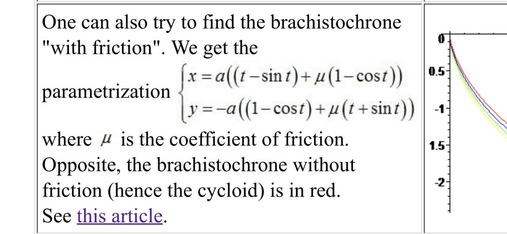
Text reading "One can also try to find the brachistochrone with friction" with the parametrization x = a((t - sin t) + mu(1 - cos t)), y = -a((1 - cos t) + mu(t + sin t)), and a graph of several curves descending from the origin.


from:
https://mathcurve.com/courbes2d.gb/brachistochrone/brachistochrone.shtml

@etotheipi
 
Last edited:
This was already explained in the linked article. To summarise, imagine the particle as bead sliding along a rail in the shape of the trajectory. The contact force ##\mathbf{N}## satisfies$$(\mathbf{N} + m\mathbf{g})\cdot \mathbf{n} = \frac{mv^2}{\rho} \mathbf{n}$$If you approximate the RHS to be negligible, then$$\mathbf{F}_{f} = -\mu N \mathbf{t} = -\mu mg\cos{(\theta)} \mathbf{t}$$Apply Newton II tangentially,$$-mg\sin{(\theta)} - \mu mg \cos{(\theta)} = m\ddot{s}$$But ##\cos{(\theta)} = dx/ds## and ##\sin{(\theta)} = dy/ds##, so$$-g \frac{dy}{ds} - \mu g \frac{dx}{ds} = \ddot{s} = \dot{v}$$Now, critical step is to rewrite$$\dot{v} = \frac{dv}{ds} \frac{ds}{dt} = v\frac{dv}{ds} = \frac{1}{2} \frac{d}{ds} \left( v^2 \right)$$so that$$-2g \frac{dy}{ds} - 2\mu g \frac{dx}{ds} = \frac{d(v^2)}{ds}$$and now integrate, taking ##v(0,0) = 0##,$$-2g(y + \mu x) = v^2 \implies v = \sqrt{-2g(y+\mu x)}$$Now we can define the time functional$$T[y] = \int_0^l \frac{ds}{v} = \int_{x_0}^{x_1} \frac{\sqrt{1+y'^2}}{\sqrt{-2g(y+\mu x)}} dx$$Now you can let$$\mathcal{L} = \frac{\sqrt{1+y'^2}}{\sqrt{-2g(y+\mu x)}}$$and we now have to compute ##\mathcal{L}_{y}## and ##\mathcal{L}_{y'}##, and use the Euler-Lagrange condition for extremum ##\mathcal{L}_{y} = \frac{d}{dx} {\mathcal{L}}_{y'}##, i.e.$$\frac{g\sqrt{1+(y')^2}}{(-2g(y+\mu x))^{\frac{3}{2}}} = \frac{d}{dx} \left( \frac{y'}{\sqrt{(1+y'^2)} \sqrt{-2g(y+\mu x)}} \right)$$ $$\frac{g\sqrt{1+(y')^2}}{(-2g(y+\mu x))^{\frac{3}{2}}} =

\frac{
\sqrt{1+(y')^2} \sqrt{-2g(y+\mu x)} y'' - y' \left( y' y''\frac{\sqrt{-2g(y+\mu x)}}{\sqrt{1+(y')^2}} - g(y' + \mu)\frac{\sqrt{1+(y')^2}}{\sqrt{-2g(y+\mu x)}} \right)
}{
(1+y'^2)(-2g(y + \mu x))
}

$$Now we must find a substitution to make this equation more manageable!
 
  • Like
Likes   Reactions: Devin-M
You can actually simplify it fairly nicely, first multiply through by ##(-2g(y+\mu x))^{\frac{3}{2}}(1+y'^2)^{\frac{3}{2}}##, and you get$$g(1+y'^2)^2 = y''(1+y'^2)(-2g(y+\mu x)) - y'^2 y''(-2g(y+ \mu x)) - gy'(y' + \mu)(1+y'^2)$$Now regroup the ##y''## terms,$$\begin{align*}g(1+y'^2)^2 &= y'' \left[ (1+y'^2)(-2g(y+\mu x)) - y'^2(-2g(y+\mu x)\right] - gy'(y' + \mu)(1+y'^2) \\ &= -2gy''(y+\mu x) - gy'(y' + \mu)(1+y'^2)\end{align*}$$And finally transpose the second term$$g(1+y'^2) \left[ 1+2y'^2 + \mu y' \right] + 2gy''(y+\mu x) = 0$$
 
I haven’t yet managed to rearrange the formula to solve for r, ta, tb, u but just wanted to find an initial very approximate solution as a guide.

My goal was to find a curve with an approximate initial depth of -1, a horizontal distance of 1 and a nonzero u and after fiddling around for a while I got this:

https://www.desmos.com/calculator/gquh3kpggq

Screenshot of a Desmos-style graphing app showing parametric curve inputs with sliders for r = 0.29, u = 0.6, a = 2.3 and b = 4.2, and a single orange arc plotted between x of about 0.75 and 1.7 with its lowest point near y = -1.1.
 
I’ve been able to approximate the results in the linked article:

Parametric Graph: https://www.desmos.com/calculator/jkth1kofbd

Desmos graph of two cycloid-type curves descending from the origin, the orange curve above and the blue curve dipping lower, with parameter sliders for r, u, a, b, s, v, c and d listed at left.

Starting with a cycloid radius 1 with a final angle of 3.88 rad with 0 friction coefficient, I increased the friction coefficient to 0.18 and concluded it is necessary to reduce the radius from 1 to 0.845 and increase the final angle from 3.88 rad to 4.24 rad to reach approximately the same endpoint in the shortest possible time. With the added friction, the optimal path “goes deeper” than the frictionless path.
 
Last edited:
  • Like
Likes   Reactions: etotheipi
@etotheipi Is it apparent to you from your equations how to find r, ta & tb between 2 horizontal points from the coefficient of friction and the initial velocity? The math is a bit advanced for my present understanding. In the other thread (without friction) I was able to find r, ta and tb using a purely geometrical approach.

The goal is to find a “traversable path” for a vehicle similar to a magnetically levitated hyperloop in vacuum (with a certain lift to drag ratio), where the initial velocity is high enough that, even with friction, the vehicle is able to return to the starting elevation and travel from point a to horizontal point b in the shortest possible time.

For example, without friction, with 9 m/s initial velocity, a horizontal distance of 5000m can be traveled in less than 1/10th the time on the optimal path compared to the flat route.
 
Last edited:
We'd need to try an ansatz, but presumably you'd end up with the parameterisation given on the website you found. I would play around with it for a bit longer, but I'm a little bit too busy tonight 😌
 
The best I can do at this point is say here is the quickest, traversable path between horizontal points with an initial velocity and a 250:1 lift to drag ratio (0.004 coefficient of friction), but I don’t know the initial velocity or the exact horizontal distance. The start and endpoints are at the 2 intersections of the orange and blue lines (the test body starts at rest from the origin and crosses the blue line with an initial velocity and crosses again with a final velocity):

Parametric Graph: https://www.desmos.com/calculator/peb5xdtqgk

Desmos graph of a cycloid-like parametric curve descending from the origin and rising again, with a horizontal blue line at y = -5000 crossing it twice; sliders show r = 2650, u = 0.004, a = 0, b = 3.74.

Ideally I would like to find the minimum initial velocity for the optimal (for time) traversable pathway with a given horizontal distance, local gravity and coefficient of friction.
 
Last edited:
Playing around with the graph a bit more I find the minimum initial velocity for a horizontal distance of 5000m with 250:1 lift to drag ratio is equivalent to a fall down the ramp from the origin of roughly 20 meters and the optimal path for time for such a vehicle is very close to a cycloid. This gives a very rough minimum initial velocity of 19-20m/s in 9.8m/s^2 gravity or roughly ~43mph.

Graph: https://www.desmos.com/calculator/fxu9dcvmps

Desmos graphing calculator screenshot showing a cycloid-style curve, parametric in t with r = 796 and u = 0.004, dipping to about -1500 between x = 0 and about x = 4900 on a grid.


Desmos graphing app screenshot with sliders r = 796, u = 0.004, a = 0, b = 6.3, a parametric curve plotted in orange falling steeply from the origin, and a horizontal line at y = -20.

Screenshot of a Desmos graphing calculator showing a parametric cycloid-style curve (orange) with sliders for r = 796, u = 0.004, a = 0, b = 6.3, and a horizontal line at y = -20 (blue), plotted on a grid with x-axis from about 5000 to 5003 and y-axis from -19 to -23.
 
With a given r and u, is it possible to determine the y position of the cusp on the right hand side, use that to determine the initial velocity at the same depth from the cusp at the origin on the left hand side, and use that to calculate the travel time with minimal initial velocity?