Ackbach
Gold Member
MHB
- 4,148
- 94
1. Prerequisites
Before you study calculus, it is important that you have a mastery of the concepts that come before it. I found calculus difficult to master (I basically had to take Differential and Integral Calculus three times in a row!), and I think many students also find it challenging - challenging, but doable. However, if you do not have the underlying concepts down, you will find it next to impossible. Here is a list of things you should be able to do well:
1. http://www.mathhelpboards.com/threads/1385-Algebra-Do-s-and-Don-t-s and know valid algebra techniques. Algebra doesn't go away when you study calculus! If anything, calculus packs down your algebra. You'll be doing plenty of it in calculus, so make sure you're up on it.
2. http://www.mathhelpboards.com/threads/35-Trigonometry-to-Memorize-and-Trigonometry-to-Derive. The vast majority of calculus courses assume you've already had trigonometry, and will differentiate trig functions, integrate trig functions, and in various ways manipulate trig functions. You should be very comfortable with them.
3. Know some basic geometry. You should know areas of basic figures like rectangles, circles, trapezoids, etc.
2. Overview
Calculus is about change: how does one quantity change compared with another quantity? Calculus studies change by solving two problems: finding tangent lines to curves, and finding areas under curves. One of the most powerful theorems in existence, the Fundamental Theorem of the Calculus, shows that solving these two problems are inverse procedures, the one of the other. The Fundamental Theorem of the Calculus is responsible for the modern... technological... age. It's nearly impossible to overestimate its importance. Without it, the computer on which I'm typing this up would not exist. Neither would air conditioning, cars, and many, many technologies many of us now take for granted.
2.1 Overview of Tangent Lines to Curves
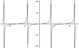
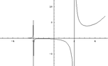
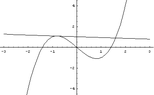
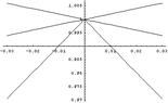
Many students are misled, I find, in their geometry courses when they're taught what a tangent line is. I hear a lot, "A tangent line to a curve is a line that touches at only one point." Indeed? What about this:
https://www.physicsforums.com/attachments/249._xfImport
Is the straight line not a tangent line to the function at $-4/5$ simply because it also intersects around $1.6$?
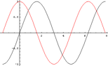
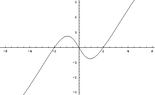
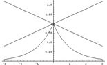
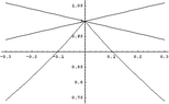
Or what about this:
https://www.physicsforums.com/attachments/250._xfImport
There's a "corner" right at $x=0$ for the graph of this function. Which "tangent line" shall we say is really tangent there? There seem to be many more than one candidate.
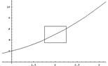
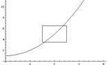
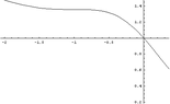
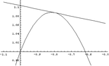
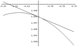
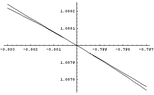
Evidently, we need to change our concept of what a tangent line is. One of the more important ideas relating to tangent lines is that this is a local phenomenon. This avoids the first issue I raised above, since the second intersection is not "right next to" where we would like to call it a tangent line. As for the second issue, let's take the first graph and zoom in a few times to see what's really happening:
https://www.physicsforums.com/attachments/251._xfImporthttps://www.physicsforums.com/attachments/252._xfImporthttps://www.physicsforums.com/attachments/253._xfImport
As you can see, the tangent line and the original function are starting to "merge" - it's almost as if they are starting to look like the same curve. If, on the other hand, we zoom in on the corner example, as follows:
https://www.physicsforums.com/attachments/254._xfImporthttps://www.physicsforums.com/attachments/255._xfImport,
we find that the picture doesn't change much. Certainly, there's no "merging" going on. So there's a fundamental difference between these two examples. We will explore that difference more when we get to derivatives.
2.2 Overview of Areas Under Curves
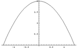
If you've paid attention to the prerequisites I mentioned earlier, you should know how to calculate the area of a rectangle, a trapezoid, and a circle. But how would you compute the area under a parabola? There's not a nice, neat, geometric formula for that (as yet!). However, solving the problem is important for many reasons. Here's an example:
https://www.physicsforums.com/attachments/248._xfImport
The function is $f(x)=-x^{2}+2$, and we'd like to know the area under this curve from $-\sqrt{2}$ to $+\sqrt{2}$. How to find it?
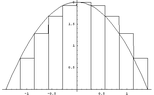
Well, if a problem is too hard, try to break it down into smaller pieces. And that's exactly what we do here. Try fitting rectangles to this curve, and compute the areas of those rectangles. So, you could try one rectangle with a height of $2$, and width $2\sqrt{2}$. You'd get an area of $4\sqrt{2}$. But you know that would overestimate the desired area. You could do better by trying two rectangles, and maybe use the value of the function in the middle of each subinterval for a rectangle height.
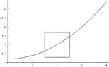
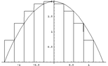
Here's a graphical illustration of using 10 rectangles with left-hand endpoints.
https://www.physicsforums.com/attachments/256._xfImport.
Here's a graphical illustration of using 10 rectangles with right-hand endpoints.
https://www.physicsforums.com/attachments/258._xfImport.
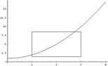
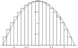
Finally, here's an example of using 20 rectangles with right-hand endpoints. You can see that the area is more accurately represented with more rectangles.
https://www.physicsforums.com/attachments/259._xfImport
Underlying both procedures (finding tangent lines and finding areas under curves) is the concept of the limit. For the tangent line problem, we are essentially going to be taking the limit of slopes of secant lines. For the area problem, we're going to take the limit as the number of rectangles goes to infinity. It is to the concept of limit that we turn first.
Comments and questions should be posted here:
http://mathhelpboards.com/commentary-threads-53/commentary-differential-calculus-tutorial-4228.html
Before you study calculus, it is important that you have a mastery of the concepts that come before it. I found calculus difficult to master (I basically had to take Differential and Integral Calculus three times in a row!), and I think many students also find it challenging - challenging, but doable. However, if you do not have the underlying concepts down, you will find it next to impossible. Here is a list of things you should be able to do well:
1. http://www.mathhelpboards.com/threads/1385-Algebra-Do-s-and-Don-t-s and know valid algebra techniques. Algebra doesn't go away when you study calculus! If anything, calculus packs down your algebra. You'll be doing plenty of it in calculus, so make sure you're up on it.
2. http://www.mathhelpboards.com/threads/35-Trigonometry-to-Memorize-and-Trigonometry-to-Derive. The vast majority of calculus courses assume you've already had trigonometry, and will differentiate trig functions, integrate trig functions, and in various ways manipulate trig functions. You should be very comfortable with them.
3. Know some basic geometry. You should know areas of basic figures like rectangles, circles, trapezoids, etc.
2. Overview
Calculus is about change: how does one quantity change compared with another quantity? Calculus studies change by solving two problems: finding tangent lines to curves, and finding areas under curves. One of the most powerful theorems in existence, the Fundamental Theorem of the Calculus, shows that solving these two problems are inverse procedures, the one of the other. The Fundamental Theorem of the Calculus is responsible for the modern... technological... age. It's nearly impossible to overestimate its importance. Without it, the computer on which I'm typing this up would not exist. Neither would air conditioning, cars, and many, many technologies many of us now take for granted.
2.1 Overview of Tangent Lines to Curves
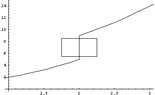
Many students are misled, I find, in their geometry courses when they're taught what a tangent line is. I hear a lot, "A tangent line to a curve is a line that touches at only one point." Indeed? What about this:
https://www.physicsforums.com/attachments/249._xfImport
Is the straight line not a tangent line to the function at $-4/5$ simply because it also intersects around $1.6$?
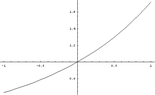
Or what about this:
https://www.physicsforums.com/attachments/250._xfImport
There's a "corner" right at $x=0$ for the graph of this function. Which "tangent line" shall we say is really tangent there? There seem to be many more than one candidate.
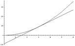
Evidently, we need to change our concept of what a tangent line is. One of the more important ideas relating to tangent lines is that this is a local phenomenon. This avoids the first issue I raised above, since the second intersection is not "right next to" where we would like to call it a tangent line. As for the second issue, let's take the first graph and zoom in a few times to see what's really happening:
https://www.physicsforums.com/attachments/251._xfImporthttps://www.physicsforums.com/attachments/252._xfImporthttps://www.physicsforums.com/attachments/253._xfImport
As you can see, the tangent line and the original function are starting to "merge" - it's almost as if they are starting to look like the same curve. If, on the other hand, we zoom in on the corner example, as follows:
https://www.physicsforums.com/attachments/254._xfImporthttps://www.physicsforums.com/attachments/255._xfImport,
we find that the picture doesn't change much. Certainly, there's no "merging" going on. So there's a fundamental difference between these two examples. We will explore that difference more when we get to derivatives.
2.2 Overview of Areas Under Curves
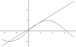
If you've paid attention to the prerequisites I mentioned earlier, you should know how to calculate the area of a rectangle, a trapezoid, and a circle. But how would you compute the area under a parabola? There's not a nice, neat, geometric formula for that (as yet!). However, solving the problem is important for many reasons. Here's an example:
https://www.physicsforums.com/attachments/248._xfImport
The function is $f(x)=-x^{2}+2$, and we'd like to know the area under this curve from $-\sqrt{2}$ to $+\sqrt{2}$. How to find it?
Well, if a problem is too hard, try to break it down into smaller pieces. And that's exactly what we do here. Try fitting rectangles to this curve, and compute the areas of those rectangles. So, you could try one rectangle with a height of $2$, and width $2\sqrt{2}$. You'd get an area of $4\sqrt{2}$. But you know that would overestimate the desired area. You could do better by trying two rectangles, and maybe use the value of the function in the middle of each subinterval for a rectangle height.
Here's a graphical illustration of using 10 rectangles with left-hand endpoints.
https://www.physicsforums.com/attachments/256._xfImport.
Here's a graphical illustration of using 10 rectangles with right-hand endpoints.
https://www.physicsforums.com/attachments/258._xfImport.
Finally, here's an example of using 20 rectangles with right-hand endpoints. You can see that the area is more accurately represented with more rectangles.
https://www.physicsforums.com/attachments/259._xfImport
Underlying both procedures (finding tangent lines and finding areas under curves) is the concept of the limit. For the tangent line problem, we are essentially going to be taking the limit of slopes of secant lines. For the area problem, we're going to take the limit as the number of rectangles goes to infinity. It is to the concept of limit that we turn first.
Comments and questions should be posted here:
http://mathhelpboards.com/commentary-threads-53/commentary-differential-calculus-tutorial-4228.html
Attachments
-
 AreaEx1.PNG953 bytes · Views: 455
 -
 TangentEx1.PNG859 bytes · Views: 479
 -
 TangentEx2.PNG1.5 KB · Views: 482
 -
 TangentEx3a.PNG1.2 KB · Views: 456
 -
 TangentEx3b.PNG1.2 KB · Views: 463
 -
 TangentEx4b.PNG1.4 KB · Views: 466
 -
 TangentEx4a.PNG1.4 KB · Views: 454
 -
 TangentEx3c.PNG1 KB · Views: 478
 -
 AreaEx2.PNG1.2 KB · Views: 456
 -
 AreaEx3.PNG1.1 KB · Views: 474
 -
 AreaEx4.PNG1.3 KB · Views: 485
Last edited by a moderator: