Leureka
- 34
- 4
- TL;DR
- Can a phase property explain violation of bell's inequality?
Hi there, i must preface with saying my understanding of the problem is limited to undergraduate quantum mechanics, since my spacialization is chemistry. I know the basic principles, like hilbert spaces, vector bases etc... I'm only asking this question because i genuinely want to understand where my thinking goes wrong.
I'm struggling to completely wrap my head around Bell's tests with polarization of photons. Popular videos always explain this with showing very simple tables of possible measurement outcomes, with a net probability for each photon passing being proportional to the square of the cosine of the angle between polarizers (Malus' law, basically), and showing how this probability distribution is fundamentally incompatible with hidden variables on each photon, determining beforehand wether it will pass or not.
It is my understanding that each time a photon arrives at one of the detectors, there is fundamentally a 50/50 chance the detector will blip or not. It is only when I combine my results with those from the other detector that i will see there actually is a correlation between the results, and this will depend on the angle between the detectors, which on a surface level seems spooky because how can each photon know what the other photon did, as to preserve the correlations?
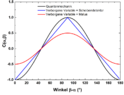
For example, for angles at 22.5 degrees there is an overall 85% correlation. Which means, in a set of 10 measurements, around 8 of them will be the same, even though at each detector the total distribution is 50%, like in the image below.

But here's an explanation which involves entirely local variables that can come up with the exact same distribution.
Imagine a vector in a circle. With respect to the horizontal, this vector can take on any angle from 0 to 360 degrees. This can represent some kind of hidden phase the two entangled photons have in common (in the image below, one is colored yellow and another is red; these are just different independent vectors, as if they were on different pairs of photons).
Now what happens at the moment of measurement? There is an angle choice, but no matter what this angle choice is, there will always be a 50% chance to measure the photon. I represented this by coloring half the circle in blue. If the phase vector lands inside the blue area, the detector will blip. What the angle choice does, is rotate the circle. The phase vector is invariant, but it has a definite inclination with the respect to the measurement angle, which is simply the horizontal cutting the circle in two.
The only nuance is that the angle inclination is not linear: so at 0 degrees the two horizontals are the same, but at 45 degrees the horizontal are perpendicular, at 22.5 it is at 15 degrees from the horizontal, and so on. The important point is that the probability is given by the overlap of the blue areas. (note that here the 22.5 is not the correct angle only for ease of drawing)

There is clearly nothing spooky in this setup. The only issue is that it's not clear to me what the circle actually represents, but whatever it is it is a property of the detector, which is nonlinear but still local. From the looks of my diagram, it seems as if the detectors also have a certain "phase", and interaction only happens when both phases are compatible. Here I chose to picture the phase of the first detector always the same for simplicity, but you could rotate it and still get the same result (if you also rotate the other circle by the same amount, which is akin to keeping the angle difference the same). In this sense there is no absolute detector phase, the only constraint is that they must be the same for polarizers at the same angle, which makes sense since they should be, in principle, indistinguishable. As for the non-linearity, I havent really thought too much on how to explain that away, but it eerely reminds me of the relationship between quaternions, which is also non-linear. Here's another analogy: replace the two circles with two ellipses. Now rotate one. The overlap is not linear anymore (see below). An ellipse in general does not reproduce a cosine dependence, but you can just pick a shape that will, it's a matter of geometricizing the problem imho.

Here, the red area represent the overlap between the two ellipses. As you can see, it does not decrease linearly as the ellipse rotates.
In essence, the correlations are an interplay between the state of the photons and the state of the detector.
Comments anyone? Where did i go wrong? Are my assumptions incorrect for example? Did I misunderstand experimental results?
I'm struggling to completely wrap my head around Bell's tests with polarization of photons. Popular videos always explain this with showing very simple tables of possible measurement outcomes, with a net probability for each photon passing being proportional to the square of the cosine of the angle between polarizers (Malus' law, basically), and showing how this probability distribution is fundamentally incompatible with hidden variables on each photon, determining beforehand wether it will pass or not.
It is my understanding that each time a photon arrives at one of the detectors, there is fundamentally a 50/50 chance the detector will blip or not. It is only when I combine my results with those from the other detector that i will see there actually is a correlation between the results, and this will depend on the angle between the detectors, which on a surface level seems spooky because how can each photon know what the other photon did, as to preserve the correlations?
For example, for angles at 22.5 degrees there is an overall 85% correlation. Which means, in a set of 10 measurements, around 8 of them will be the same, even though at each detector the total distribution is 50%, like in the image below.
But here's an explanation which involves entirely local variables that can come up with the exact same distribution.
Imagine a vector in a circle. With respect to the horizontal, this vector can take on any angle from 0 to 360 degrees. This can represent some kind of hidden phase the two entangled photons have in common (in the image below, one is colored yellow and another is red; these are just different independent vectors, as if they were on different pairs of photons).
Now what happens at the moment of measurement? There is an angle choice, but no matter what this angle choice is, there will always be a 50% chance to measure the photon. I represented this by coloring half the circle in blue. If the phase vector lands inside the blue area, the detector will blip. What the angle choice does, is rotate the circle. The phase vector is invariant, but it has a definite inclination with the respect to the measurement angle, which is simply the horizontal cutting the circle in two.
The only nuance is that the angle inclination is not linear: so at 0 degrees the two horizontals are the same, but at 45 degrees the horizontal are perpendicular, at 22.5 it is at 15 degrees from the horizontal, and so on. The important point is that the probability is given by the overlap of the blue areas. (note that here the 22.5 is not the correct angle only for ease of drawing)
There is clearly nothing spooky in this setup. The only issue is that it's not clear to me what the circle actually represents, but whatever it is it is a property of the detector, which is nonlinear but still local. From the looks of my diagram, it seems as if the detectors also have a certain "phase", and interaction only happens when both phases are compatible. Here I chose to picture the phase of the first detector always the same for simplicity, but you could rotate it and still get the same result (if you also rotate the other circle by the same amount, which is akin to keeping the angle difference the same). In this sense there is no absolute detector phase, the only constraint is that they must be the same for polarizers at the same angle, which makes sense since they should be, in principle, indistinguishable. As for the non-linearity, I havent really thought too much on how to explain that away, but it eerely reminds me of the relationship between quaternions, which is also non-linear. Here's another analogy: replace the two circles with two ellipses. Now rotate one. The overlap is not linear anymore (see below). An ellipse in general does not reproduce a cosine dependence, but you can just pick a shape that will, it's a matter of geometricizing the problem imho.
Here, the red area represent the overlap between the two ellipses. As you can see, it does not decrease linearly as the ellipse rotates.
In essence, the correlations are an interplay between the state of the photons and the state of the detector.
Comments anyone? Where did i go wrong? Are my assumptions incorrect for example? Did I misunderstand experimental results?
Last edited: