From what I have seen,
Bondi's "k-calculus" (which is an algebra-based method) is the simplest approach for introducing special relativity, with the emphasis kept on the relativity principle, the invariance of the speed of light, and spacetime geometry (on a position-vs-time graph)... motivated by operational definitions.
The usual Lorentz Transformation formula are seen as a secondary consequence of the approach.
(This is because Bondi works in the eigenbasis of the Lorentz boost transformation.
One has to re-write his equations in terms of rectangular coordinates to the more recognizable formula.)
Here is my Insight on this approach (providing more details that what Bondi presents to a general audience)
https://www.physicsforums.com/insights/relativity-using-bondi-k-calculus/ ,
which underlies my Relativity on Rotated Graph Paper approach.
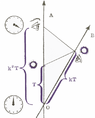
The proper-times are related by
\begin{align}
\tau_{OE}& =k \tau_{OC}\\
\tau_{ON}& =k\tau_{OE}=k^2\tau_{OC}
\end{align}
where the relativity principle implies the same value of ##k##.
[##k## started out as just a proportionality constant for each observer,
but now are equal according to relativity
...it's more-familiar physical interpretation is uncovered later.]
These will be called the "radar coordinates of E (with origin at O)" ##u=\tau_{ON}## and ##v=\tau_{OC}##. (##v## is not a velocity.)
If you are just interested in the Lorentz Transformation,
you can skip some of these beginning subsections (intended for physical interpretation and connection with standard textbook formulas).
- [To interpret in terms of rectangular coordinates...]
The lab frame uses the "radar-method" to assign rectangular coordinates, where ##\tau_{OC}## is the clock-reading when the lab frame sends a light-signal to event E and ##\tau_{ON}## is the clock-reading when the lab frame receives a light-signal from event E \begin{align}
\Delta t_{OE}&=\frac{1}{2}(\tau_{ON} + \tau_{OC})=\frac{1}{2}(k^2T + T)\\
\Delta x_{OE}/c&=\frac{1}{2}(\tau_{ON} - \tau_{OC})=\frac{1}{2}(k^2T - T)
\end{align}
[This is arguably more-physical and more-practical for astronomical observations.
(No long rulers into space are needed.
No distant clocks at rest with respect to the observer are needed.)]
(The first of this pair displays "time-dilation" when compared to ##\tau_{OE}=kT##.)
- [To interpret ##k## terms of the relative velocity ##V##...]
By division, we get a relation between the relative-velocity ##V## and ##k## (which turns out to be the Doppler formula)
\begin{align}
V_{OE}&=\frac{\Delta x_{OE}}{\Delta t_{OE}}=\frac{\frac{1}{2}c(k^2T – T)}{\frac{1}{2}(k^2T + T)}=\frac{k^2-1}{k^2+1}c
\end{align}
- [To recognize the square-interval in rectangular form...]
Instead, by addition and subtraction,
we get
\begin{align}
\tau_{ON} &=\Delta t_{OE}+\Delta x_{OE}/c=k^2T\\
\tau_{OC} &=\Delta t_{OE}-\Delta x_{OE}/c=T
\end{align}
so we see that their product is invariant (to be called the "squared-interval of OE") and is equal to the square-of-the-proper-time along OE
\begin{align}
\tau_{ON} \tau_{OC} &=\Delta t_{OE}^2-(\Delta x_{OE}/c)^2=(kT)^2=\tau_{OE}^2
\end{align}
- Again, with these "radar coordinates" ##u=\tau_{ON}## and ##v=\tau_{OC}##, we can locate event E. (Note: ##v## is not a velocity.)
To obtain the Lorentz-Transformation and the Velocity-Transformation,
introduce another observer (Brian) and compare the proper-times along Brian's worldline
with what was obtained along the Lab Frame (Alfred): ##\tau_{ON}## and ##\tau_{OC}##.
We can see that Alfred and Brian's radar-coordinates for event E are related by:
$$
\begin{align}
u &= k_{AB} u'\\
v' &= k_{BA} v.
\end{align}
$$
By the relativity-principle, ##k_{AB}=k_{BA}##. So, call it ##K_{rel}##.
Rewriting as
$$
\begin{align}
u' &= \frac{1}{K_{rel}} \ u\\
v' &= K_{rel} \ v,
\end{align}
$$
we have the Lorentz Transformation in radar coordinates (i.e. in the eigenbasis).
(Clearly, ##u'v'=uv##... displaying the invariance of the interval along OE.)
No time-dilation factor ##\gamma=\frac{1}{\sqrt{1-(V/c)^2}}## or velocity ##V## is needed
... just the Doppler factor $K$.
- To obtain the Lorentz transformation in rectangular coordinates...:
do addition and subtraction (and dropping the ##{}_{rel}## subscript),
$$
\begin{align}
u' +v' &= ( \frac{1}{K} \ u) + (K \ v ) \\
u' - v' &= ( \frac{1}{K} \ u) + (K \ v )
\end{align}
$$
Then, introducing the rectangular coordinates (dropping the ##\Delta##s) we have:
\begin{align}
2 t' &= ( \frac{1}{K} \ (t+x/c) ) + (K \ (t-x/c) ) = (K+\frac{1}{K})t - (K-\frac{1}{K})x/c \\
2 x'/c &= ( \frac{1}{K} \ (t+x/c) ) + (K \ (t-x/c) ) = -(K-\frac{1}{K} )t + (K+\frac{1}{K})x/c
\end{align}
Some algebra shows that the time-dilation factor ##\gamma=(K+\frac{1}{K})/2##
and ##\gamma V=(K-\frac{1}{K})/2##. This is easier if one writes ##K=e^\theta## and
observes that ##V=c\tanh\theta## and ##\gamma=\cosh\theta##.
The Lorentz Transformation in radar-coordinates involves the Doppler Factor and is mathematically simpler (since the equations for its coordinates are uncoupled)
compared to
the Lorentz Transformation in rectangular-coordinates, which involves the time-dilation factor and the velocity.
Physically, ##K## is simpler to measure.
Assuming these zero their clocks at their meeting...
As a light-signal is sent, send the image of the sender's clock.
When a signal is received, compare the sender's transmitted image of his clock at sending
with the receiver's clock there at receiving. The ratio of reception to emission is ##K##.
But they don't have to meet or zero their clocks.
Just send two signals... and work with differences.