Killing sinusoidal baseline in spectrum

In summary, the amplitude levels of the peaks in the spectra may vary depending on the bandwidth of the receive filter, and it may be difficult to eliminate the variation.
  • #1
jolindbe
12
0
Hi,
I have a bunch of spectra which happen to show some sinusoidal baselines, like this:
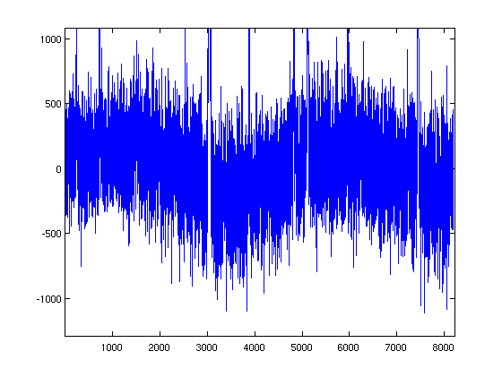
35jf66q.jpg


I would like to subtract these baselines somehow. Of course I can try to fit sinusoidals using for instance Matlab's lsqcurvefit, but it seems like I have to be very careful with my input guesses not to get completely insane results, which makes it very tedious for my spectra.

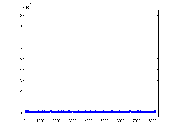
So I thought that I could do something about it in Fourier space instead. Just to try it out, I first made some dummy data (sinusoidal with similar frequency as in real data + Gaussian noise, no spectral lines), to see what that looks like in Fourier space:
Code:
N=8192;
t=1:N;
sinf = 250*sin(0.00135*t);
wanted_data = random('Normal',0,100,1,N);
data = sinf+wanted_data;
fftdata = fft(data)

1zbx6pl.png


As you can see above, abs(fftdata) shows two very prominent spikes just on the edges of the spectrum, which sounds reasonable. The Fourier transform of a sine wave would be two dirac-deltas, and they should appear far out when the frequency is low compared to the spectral window. Let's try to kill it:

Code:
fft_approx = zeros(1,N);
fftdata = fft(data);
for i = 1:N
    if abs(fftdata(i)) < 1e5
        fft_approx(i) = 0;
    else
        fft_approx(i) = fftdata(i);
    end
end

result_data = ifft(fftdata-fft_approx);

So above I have extracted the really high-amplitude parts of the Fourier spectrum, and subtracted them from the fft of the data, and taken the inverse fft of this. The result is fairly similar to wanted_data, and if I plot the difference of these I get this:
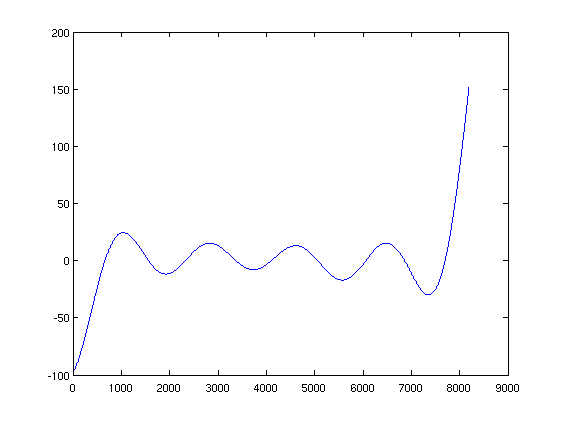
swe33k.jpg


A new (higher-frequency) sine wave, but with a much lower amplitude than the original (by a factor of 10). Ok, it's not perfect, but this might actually work...

Let's make a try on the real data. The absolute value of the fft of the data looks like this:
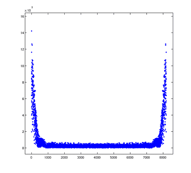
2q1xjcg.jpg


The features on the sides are much wider. How do I get rid of this? I have tried two methods:

Method 1: Subtracting all data with abs(fftdata) higher than a certain value (as above):

Code:
fft_approx = zeros(1,N);
fftdata = fft(data);
highval = 2e5;
for i = 1:N
    if abs(fftdata(i)) < highval
        fft_approx(i) = 0;
    else
        fft_approx(i) = fftdata(i);
    end
end
result_data = ifft(fftdata-fft_approx);

Method 2: Fitting polynomials to the outer edges, subtracting data scaled with this polynomial:

Code:
fft_pol = zeros(1,N);
fftdata = fft(data);

nlim = 500;
degree = 3;
p1 = polyfit(t(1:nlim),abs(fftdata(1:nlim)),degree);
p2 = polyfit(t(N-nlim:N),abs(fftdata(N-nlim:N)),degree);
for k = 1:N
    if k <= nlim
        fft_pol(k) = 1*polyval(p1,k)*fftdata(k)/abs(fftdata(k));
    else
        if k >= N-nlim+1
            fft_pol(k) = 1*polyval(p1,N-k+1)*fftdata(k)/abs(fftdata(k));
        else
            fft_pol(k) = 0;
        end
    end
end

result_data = ifft(fftdata-fft_pol);

I can modify highval in Method 1, and nlim and degree in Method 2. But fiddling with the parameters does not produce great results, it seems like I either get very little result on my baseline, or that my signal-to-noise decreases a lot. Sometimes I get a different sinusoidal in my baseline instead (with much higher frequency).

Does anybody have a clue on how to treat that kind of data in the Fourier domain, or is the best way of solving it simply to give in and fit sinusoidals?

EDIT: My code above is in Matlab, but I also speak Python/numpy/scipy...
 
Last edited:
Engineering news on Phys.org
  • #2
If I'm not missing something, you could just pass your waveform through a suitable high-pass filter?
 
  • #3
Firstly, are you sure that the apparent variation is or is not an artifact of the measuring system? Apart from the obvious reason of eliminating those 'bumps' - to produce a nice picture - , have you questioned the validity of what you're trying to do with that data?
What do those bumps actually represent? They are pretty massive to say that you just want to 'get rid of them'. They may be very significant and they aren't just a variation of the "baseline" they are variation in the amplitudes of the peaks too.

Do the bumps appear in the same places for different measurement runs? Can you be certain that they really correspond to an 'added signal' - which would have to consist of a frequency dependent spectrum of wideband noise (?) which has a similar amplitude to your wanted signal?
The amplitude values are a function of the bandwidth of the receive filter. If there is some modulation of the received signals that depends upon the frequency then the measured level could change. What happens if you change the IF bandwidth of the analyser? Perhaps you have to deal with data that's already been presented to you and you can't experiment.
 
  • #4
sophiecentaur said:
Firstly, are you sure that the apparent variation is or is not an artifact of the measuring system? Apart from the obvious reason of eliminating those 'bumps' - to produce a nice picture - , have you questioned the validity of what you're trying to do with that data?
What do those bumps actually represent? They are pretty massive to say that you just want to 'get rid of them'. They may be very significant and they aren't just a variation of the "baseline" they are variation in the amplitudes of the peaks too.

The sinusoidal baseline is an artifact. This is radio astronomy data, and a non-flat baseline does not make sense. The receiver people at the telescope are aware of the problem, and the telescope is nowadays producing nice flat baselines - but my data are from before that was fixed, and they simply recommend me to fit a sinusoidal baseline, or linear baselines for each spectral line.

sophiecentaur said:
Do the bumps appear in the same places for different measurement runs? Can you be certain that they really correspond to an 'added signal' - which would have to consist of a frequency dependent spectrum of wideband noise (?) which has a similar amplitude to your wanted signal?
The amplitude values are a function of the bandwidth of the receive filter. If there is some modulation of the received signals that depends upon the frequency then the measured level could change. What happens if you change the IF bandwidth of the analyser? Perhaps you have to deal with data that's already been presented to you and you can't experiment.

The bumps change over the different scans. I don't know the exact source of the issue, but since the receiver people recommends subtracting the baseline, I am assuming that they know what they are talking about.

I unfortunately cannot get any new data, this is what I have...

milesyoung said:
If I'm not missing something, you could just pass your waveform through a suitable high-pass filter?

That makes sense... I hadn't thought about that. I'll have to check for Matlab or Python packages for that.
 
  • #5
I see. You are stuck with that data. Commiserations; you just have to make the best of it.

Milesyoung's HPF idea makes sense. I was going to suggest effectively the same thing and that is to look at the mean of the minima over a small range and use that as a baseline for the maxima in that region. Then repeat this over the whole range. It seems a bit less 'arbitrary' than trying to extract the sinusoid from those bumps and it would be very quick to try.
 
  • #6
Your baseline is extremely low frequency compared to the frequency content of the data you're interested in, so a simple one-pole high-pass filter with a cutoff more than a decade above your baseline should suffice. You have a very large margin for error in placing the cutoff.

Have a look at MATLAB's filter command. You don't need a package for it as far as I recall.
 
  • #7
First, thanks for all help so far.

sophiecentaur said:
look at the mean of the minima over a small range and use that as a baseline for the maxima in that region. Then repeat this over the whole range.

I'm sorry, but I don't really understand what you mean. How is this similar to an HPF, and what should I do with the baselines?

milesyoung said:
Your baseline is extremely low frequency compared to the frequency content of the data you're interested in, so a simple one-pole high-pass filter with a cutoff more than a decade above your baseline should suffice. You have a very large margin for error in placing the cutoff.

Have a look at MATLAB's filter command. You don't need a package for it as far as I recall.

Ok, I gave it a go. I know very little about filters (I've never really had a use for them before), but found a page claiming that I will get a high-pass filter in Matlab using this:

Code:
a=something;
filt_data=filter([1-a a-1],[1 a-1], data);

Does this make sense? I've tried to google more on it, but it seems most people recommend the use of more advanced Matlab functions, but I'd like to keep this as simple as possible.

Anyway, assuming the above version is correct, it seems like the best a parameter is around 0.01-0.2 - I get rid of the sinusoidal baseline, but the spectral lines change:

e6pwys.png

(upper pane: original, lower pane: filtered with a=0.1)

As you can see, the spectral lines now are fainter, but have a negative component at a slightly higher position. If I increase a, I sooner or later attenuate everything, if I decrease a, I first get wider negative things, and then I am back at my original spectrum.

I suppose the problem is in my filter, but I don't really know how to modify it in a sensible way.
 
  • #8
jolindbe said:
First, thanks for all help so far.

I'm sorry, but I don't really understand what you mean. How is this similar to an HPF, and what should I do with the baselines?
Looking at your original data, I am not too sure what the Y axis scale represents (there's no label you naughty boy! :wink:) I was assuming that it was a power spectrum and the Y scale was some sort of logarithmic scale (hence the + and - signs), which is what you would normally present a spectrum(?). I, hence, was assuming that, in the absence of signal and with low noise, there would be a straight fuzzy base line somewhere along the lower half of the plot. The bumps would suggest that the noise is somehow modulated during the frequency sweep.
It would be nice to sort this out - if only to indulge me!
 
  • #9
Ah, your waveform has low frequency components (down to DC). The high-pass filter is working as intended - it just knocks out those components as well so it'll corrupt your data.
 
  • #10
milesyoung said:
Ah, your waveform has low frequency components (down to DC). The high-pass filter is working as intended - it just knocks out those components as well so it'll corrupt your data.

Isn't the X axis 'frequency'? We don't know for sure until he tells us what the axes actually are. I can't see what it all means until that's cleared up.
The bumps could be due to 'hum' modulating the signal at RF or IF or they could be due to a standing wave pattern in a feeder. They seem to represent a spurious amplitude variation with frequency (/plot sweep).
 
  • #11
sophiecentaur said:
Looking at your original data, I am not too sure what the Y axis scale represents (there's no label you naughty boy! :wink:) I was assuming that it was a power spectrum and the Y scale was some sort of logarithmic scale (hence the + and - signs), which is what you would normally present a spectrum(?). I, hence, was assuming that, in the absence of signal and with low noise, there would be a straight fuzzy base line somewhere along the lower half of the plot. The bumps would suggest that the noise is somehow modulated during the frequency sweep.
It would be nice to sort this out - if only to indulge me!

Haha, I agree axes should have labels, point taken ;)
The y-axis represents flux density, which is usually measured in Kelvin(!), but this is now an arbitrary unit. The x-axis represents frequency, but is now just channel number. It is all completely linear. So the detector reads off how much flux per frequency unit is emitted in each channel, which each cover some 100 kHz of the band. The x-axis goes from something like 217 GHz to 218 GHz.

Normal data would be a baseline around zero with Gaussian noise (around zero), and then some relatively narrow spectral lines here and there. Normally the lines are positive, but lines with negative flux density are also possible - that would mean an absorption line, but it is unusual in radio astronomy (more common in the optical).
 
  • #12
OK - so there isn't an actual +/- on the Y scale unless it's a log scale and you definitely can't have a -K. You can't have 'negative energy flux'- just less than you'd expect (no?).
So my original suggestion was to establish a 'local, running mean' baseline by 'averaging' a number of minima, adjacent to each sample and subtracting that value from each of the peaks to establish the height of each other sample wrt this value. That should produce a plot with a more level baseline. It is in fact quite similar low pass filtering the signal, I think but (by being non-linear) it will have less effect on the relative heights of adjacent maxima than would a simple low pass filter.
I think there may be an added advantage in a method like this because it will serve to reduce non-sinusoidal variations too.
 
  • #13
sophiecentaur said:
OK - so there isn't an actual +/- on the Y scale unless it's a log scale and you definitely can't have a -K. You can't have 'negative energy flux'- just less than you'd expect (no?).

You definitely can have a measured flux density that is negative, since your baseline is usually a black-body continuum (which can be assumed to be flat at these relatively narrow bands). And the noise is fluctuating around zero, equally many wiggles below as above. These are simply fluctuations from the black-body curve (mainly due to noise in your instrument), which is the baseline.

Edit: And, no, it is not a log scale.

sophiecentaur said:
So my original suggestion was to establish a 'local, running mean' baseline by 'averaging' a number of minima, adjacent to each sample and subtracting that value from each of the peaks to establish the height of each other sample wrt this value. That should produce a plot with a more level baseline. It is in fact quite similar low pass filtering the signal, I think but (by being non-linear) it will have less effect on the relative heights of adjacent maxima than would a simple low pass filter.
I think there may be an added advantage in a method like this because it will serve to reduce non-sinusoidal variations too.

Since the noise should average around zero your suggestion will not work. However, it could be modified. I could estimate a local running mean of all data points (ideally excluding the spectral lines without knowing the baseline as a prior, but that shouldn't be impossible). I'll give it a try...
 
Last edited:
  • #14
I guess we're just talking in different terms. It has to be true that you can't have a negative flux of energy but, of course, you can say that a given flux is less than a reference value - which is where your negative values come from. I guess it is convenient to use in those circs.

The minima on your plot do not fall to zero though, they fall below the zero on your scale. (This is what is giving my brain a problem) But how can any receiver give an output value less than its own noise floor? What value of plot would be expected if you pointed the telescope at the quitest spot you could find in space? Zero on your graph?? That would make no sense to me at all. Where does the receiver noise floor come on that graph?
Problem for me is looking in on a totally unfamiliar discipline and the lingo gets n my way.
 
  • #15
sophiecentaur said:
I guess we're just talking in different terms. It has to be true that you can't have a negative flux of energy but, of course, you can say that a given flux is less than a reference value - which is where your negative values come from. I guess it is convenient to use in those circs.

The minima on your plot do not fall to zero though, they fall below the zero on your scale. (This is what is giving my brain a problem) But how can any receiver give an output value less than its own noise floor? What value of plot would be expected if you pointed the telescope at the quitest spot you could find in space? Zero on your graph?? That would make no sense to me at all. Where does the receiver noise floor come on that graph?
Problem for me is looking in on a totally unfamiliar discipline and the lingo gets n my way.

I also thought this was a bit confusing when I was new to radio astronomy (and then I got used to it...). If I would look at a completely blank spot on the sky, I would get noise around zero (positive and negative). If I take a very short integration, the noise would have large amplitude around zero, but as the integration time passes by, the noise level goes down, but still centred around zero.

I think that this noise stems from the receiver's blackbody radiation (it is usually cooled by liquid helium, but even that has a T > 0 K). If I remember correctly, the receiver produces a voltage (positive or negative) for each channel, stating the difference between the signal and the normal noise level of the receiver. This voltage is then converted to a value in Kelvin, or Jansky, depending on your preference.
 
  • #16
Short version: I think that I've found an acceptable solution to the problem, thanks to the suggestions from sophiecentaur!

I made a code (now in Python, since it's more comfortable to me) that creates a baseline from the mean of a group of channels for each channel. The mean is weighted by a Gaussian peaking at the channel for which the mean is taken, so that the neighbouring channels contribute more than those far away.

For anyone interested, here's the code:

Code:
from matplotlib import pyplot as plt
import numpy

def gauss(mu, sigma, x ) :
    return (1.0/(sigma*numpy.sqrt(2*numpy.pi)))*numpy.exp(-(x-mu)**2/(2.0*sigma**2))

# import the data
data = something

# Flags for the spectral lines
flag_chans = [[224,249],[711,741],[2520,2540],[3006,3074],[3865,3889],[4808,4837],[5092,5133],[7421,7462]]

N=len(data)

# Create some x axis
x = numpy.array(range(N))

# A number of channels that should be large enough so that they can represent the typical inclination at a certain point in the spectrum
rn = 30

# A new array for the data where lines are removed
flagged_data = numpy.array(data)

# Remove spectral lines and replace them with a straight line
for fl in flag_chans:
    fitlinereg = []
    fitline_y = numpy.concatenate((flagged_data[fl[0]-rn:fl[0]],flagged_data[fl[1]:fl[1]+rn]))
    fitline_x = numpy.concatenate((x[fl[0]-rn:fl[0]],flagged_data[fl[1]:fl[1]+rn]))
    p = numpy.polyfit(fitline_x,fitline_y,1)
    for i in range(fl[0],fl[1]):
        flagged_data[i] = numpy.polyval(p,i)

# These constants can be modified
median_range = 900
weight_factor = 0.5

# Vector for the baseline
baseline = numpy.zeros(N)

for i in range(N):
    
    # Take care of the borders
    if i > median_range:
        ll = i-median_range
    else:
        ll = 0
    if i < N-median_range:
        ul = i+median_range
    else:
        ul = N

    # Calculate the weights
    w = gauss(i,weight_factor*median_range,numpy.array(range(ll,ul)))

    # The averaging
    baseline[i] = numpy.average(flagged_data[ll:ul],weights=w)

plt.figure()
plt.plot(x,data,'b')
plt.plot(x,baseline,'r')
plt.show()
plt.ylim(-1000,1000)

With the parameters above, the following fit is found:

n4w2kp.png


Subtraction from the data gives this baseline:

29qgtpj.png


If I modify the parameters median_range and weight_factor above, I could get a baseline that follows the data even better, but looks less sinusoidal. To avoid subtracting real stuff, I think I should be happy when the baseline is sinusoidal and follows the data.

Thanks for all the help, sophiecentaur in particular!
 
  • #17
jolindbe said:
I also thought this was a bit confusing when I was new to radio astronomy (and then I got used to it...). If I would look at a completely blank spot on the sky, I would get noise around zero (positive and negative). If I take a very short integration, the noise would have large amplitude around zero, but as the integration time passes by, the noise level goes down, but still centred around zero.

I think that this noise stems from the receiver's blackbody radiation (it is usually cooled by liquid helium, but even that has a T > 0 K). If I remember correctly, the receiver produces a voltage (positive or negative) for each channel, stating the difference between the signal and the normal noise level of the receiver. This voltage is then converted to a value in Kelvin, or Jansky, depending on your preference.

Are you talking about the noise voltage or the noise power? There is no way that you can get less noise power than the noise of your receiver/antenna, whether you specify the noise as noise temperature or Watts/Hz. To demodulate less noise than the receiver produces would require correlation between the remote source and the locally generated noise (to cause cancellation) and that's not possible. We still must be talking at cross purposes.
Could you tell me what the noise floor of your receiveing system is, compared with what is shown on that graph. Again, I have assumed you are talking about the noise power in some specified bandwidth and not Volts.
 
  • #18
sophiecentaur said:
Are you talking about the noise voltage or the noise power? There is no way that you can get less noise power than the noise of your receiver/antenna, whether you specify the noise as noise temperature or Watts/Hz. To demodulate less noise than the receiver produces would require correlation between the remote source and the locally generated noise (to cause cancellation) and that's not possible. We still must be talking at cross purposes.

I'll have to think about this and get back to you tomorrow... but I'm at least quite sure that the temperature on the y-axis is proportional to a system voltage.

sophiecentaur said:
Could you tell me what the noise floor of your receiveing system is, compared with what is shown on that graph. Again, I have assumed you are talking about the noise power in some specified bandwidth and not Volts.

The noise in my graphs is more or less purely receiver noise.
 
  • #19
What you have done has definitely successfully reduced those bumps to a level where you can't see them so it's clearly doing what you want. I agree that, if the Y scale is logarithmic, the lowest spikes are not a very significant level for reference. The mean that you've chosen seems to be pretty convincing. What do you get if you just low pass filter that data?

I assume that your spectrum analysis equipment will consist of a front end amplifier (as low a noise figure as possible), some FR filtering, a mixer then some IF filtering (two stages of IF, probably) to define the system noise bandwidth, followed by a detector. Can we agree on that basic system block diagram?

I am sure you must have misunderstood what that data actually represents if you reckon that a received signal can actually cause a reduced level of detected signal plus receiver noise. I have no direct experience of such low SNR work and there will be plenty of techniques that can be used to get the best out of a system but there are certain basic ideas about signal theory. People use all sorts of strange but valid units in specialist measuring fields. You are clearly looking for very low level signals that are narrow band and noise-like in the presence of receiver noise and using Temperature as a measure is fair enough. I just feel that the only reason to get negative values must involve a logarithmic scale. A normal spectrum analyser trace can be made to look just like yours if you jack up the gain, choose an appropriate frequency range and IF bandwidth, and use a dB scale. If you reduce the IF bandwidth (possibly introduce some baseband filtering too) and slow up the scan, this will narrow the range of the trace. I realize that you have a problem in that you are already using a pretty narrow bandwidth and your wanted signal will also be reduced by filtering (unlike CW signals in the presence of receiver noise).
 
  • #20
sophiecentaur said:
What you have done has definitely successfully reduced those bumps to a level where you can't see them so it's clearly doing what you want. I agree that, if the Y scale is logarithmic, the lowest spikes are not a very significant level for reference. The mean that you've chosen seems to be pretty convincing. What do you get if you just low pass filter that data?

Low-pass filtering the data and then subtracting that result from the data produces the same result as high-pass filtering the data (not so surprising).

sophiecentaur said:
I assume that your spectrum analysis equipment will consist of a front end amplifier (as low a noise figure as possible), some FR filtering, a mixer then some IF filtering (two stages of IF, probably) to define the system noise bandwidth, followed by a detector. Can we agree on that basic system block diagram?

Sounds fairly reasonable, I believe. This is what they call a superheterodyne receiver, if that helps. And remember, I'm an astronomer, not a telescope technician... so bear with me.

As far as I have understood, a hot and a cold load are observed by the telescope every now and then. These observations are used to establish the system temperature of the telescope. Given this information, the power or voltage from observing the sky can be converted to a "real" sky temperature. If you are observing something with a sky temperature close to 0, your output voltage will still be positive, but slightly fluctuating due to noise. This will then be converted to a sky temperature, which should be fluctuating around 0, with both positive and negative values.

sophiecentaur said:
I am sure you must have misunderstood what that data actually represents if you reckon that a received signal can actually cause a reduced level of detected signal plus receiver noise.

It is not a negative receiver signal. Normally, the source you are observing has a black-body curve with some spectral features. If you are after the spectral lines, you do not only do the corrections for the telescope temperature I mentioned above, but you also subtract this black-body curve (which is a straight line at these narrow bandwidths). It is possible to get negative features in the resulting spectra, which for instance can mean that you have optically thick gas blocking the black-body light at those wavelengths (so-called absorption lines). Your spectral lines can also have both emission and absorption components, which would tell you something about the dynamics of the gas - see for example the P Cygni profile: http://www.daviddarling.info/encyclopedia/P/P_Cygni_profile.html

sophiecentaur said:
I have no direct experience of such low SNR work and there will be plenty of techniques that can be used to get the best out of a system but there are certain basic ideas about signal theory. People use all sorts of strange but valid units in specialist measuring fields. You are clearly looking for very low level signals that are narrow band and noise-like in the presence of receiver noise and using Temperature as a measure is fair enough. I just feel that the only reason to get negative values must involve a logarithmic scale.

Not if you measure the difference between two signals, see above.
 
  • #21
jolindbe said:
Low-pass filtering the data and then subtracting that result from the data produces the same result as high-pass filtering the data (not so surprising).
Agreed - the actual characteristic of the two filters will probably be a bit different but that doesn't matter.

Sounds fairly reasonable, I believe. This is what they call a superheterodyne receiver, if that helps. And remember, I'm an astronomer, not a telescope technician... so bear with me.
Yes they will use a double conversion superhet. Good for image rejection yet still allows a narrow receive filter.
As far as I have understood, a hot and a cold load are observed by the telescope every now and then. These observations are used to establish the system temperature of the telescope. Given this information, the power or voltage from observing the sky can be converted to a "real" sky temperature. If you are observing something with a sky temperature close to 0, your output voltage will still be positive, but slightly fluctuating due to noise. This will then be converted to a sky temperature, which should be fluctuating around 0, with both positive and negative values.


It is not a negative receiver signal. Normally, the source you are observing has a black-body curve with some spectral features. If you are after the spectral lines, you do not only do the corrections for the telescope temperature I mentioned above, but you also subtract this black-body curve (which is a straight line at these narrow bandwidths). It is possible to get negative features in the resulting spectra, which for instance can mean that you have optically thick gas blocking the black-body light at those wavelengths (so-called absorption lines). Your spectral lines can also have both emission and absorption components, which would tell you something about the dynamics of the gas - see for example the P Cygni profile: http://www.daviddarling.info/encyclopedia/P/P_Cygni_profile.html

Not if you measure the difference between two signals, see above.
I'm going to have to ask for a reference about this. I have looked at a number of docs via Google and, whilst the reason for using temperature is described and justified; also the problem of distinguishing local noise from target noise etc. I have no problem with any of that but the only graphs I can find show spectra of signals from radio telescopes which have Y scales with a zero at the bottom or a log scale. This has fascinated me and I have been digging deep into my memory of noise theory. I know you're not 'wrong' but I need to understand your terms. That Y scale is very difficult to understand.
 
  • #22
sophiecentaur said:
I'm going to have to ask for a reference about this. I have looked at a number of docs via Google and, whilst the reason for using temperature is described and justified; also the problem of distinguishing local noise from target noise etc. I have no problem with any of that but the only graphs I can find show spectra of signals from radio telescopes which have Y scales with a zero at the bottom or a log scale. This has fascinated me and I have been digging deep into my memory of noise theory. I know you're not 'wrong' but I need to understand your terms. That Y scale is very difficult to understand.

Here are some spectra found by Google image search on "millimeter astronomy spectrum" or similar:

1-s2.0-S0022285212000379-gr1.jpg

l1448spec.jpg

orionthz.jpg


I could also give you links to a gazillion articles in Astronomy&Astrophysics and Astrophysics Journal using the same scale...

Perhaps parts of this text may be a good reference, even though I can't find that the author touches the subject of a baseline around zero. http://arxiv.org/pdf/1111.1183.pdf

I'm still not sure exactly on the process from antenna to output spectrum, but isn't it possible that the telescope gives a signal that is always positive, but that certain corrections in the signal processing subtracts a baseline so that the noise wiggles around zero? This would then be interpreted physically as if the signal in a certain frequency band averages to zero, there is no detection, but if the signal is stronger than, say 3sigma, there is a detection. This is the way I understand how it works, but is seems like you think this kind of processing is breaking some natural laws of signal processing... am I right?
 
  • #23
jolindbe said:
Low-pass filtering the data and then subtracting that result from the data produces the same result as high-pass filtering the data (not so surprising).


Sounds fairly reasonable, I believe. This is what they call a superheterodyne receiver, if that helps. And remember, I'm an astronomer, not a telescope technician... so bear with me.

As far as I have understood, a hot and a cold load are observed by the telescope every now and then. These observations are used to establish the system temperature of the telescope. Given this information, the power or voltage from observing the sky can be converted to a "real" sky temperature. If you are observing something with a sky temperature close to 0, your output voltage will still be positive, but slightly fluctuating due to noise. This will then be converted to a sky temperature, which should be fluctuating around 0, with both positive and negative values.


It is not a negative receiver signal. Normally, the source you are observing has a black-body curve with some spectral features. If you are after the spectral lines, you do not only do the corrections for the telescope temperature I mentioned above, but you also subtract this black-body curve (which is a straight line at these narrow bandwidths). It is possible to get negative features in the resulting spectra, which for instance can mean that you have optically thick gas blocking the black-body light at those wavelengths (so-called absorption lines). Your spectral lines can also have both emission and absorption components, which would tell you something about the dynamics of the gas - see for example the P Cygni profile: http://www.daviddarling.info/encyclopedia/P/P_Cygni_profile.html


Not if you measure the difference between two signals, see above.

jolindbe said:
Here are some spectra found by Google image search on "millimeter astronomy spectrum" or similar:

I could also give you links to a gazillion articles in Astronomy&Astrophysics and Astrophysics Journal using the same scale...

Perhaps parts of this text may be a good reference, even though I can't find that the author touches the subject of a baseline around zero. http://arxiv.org/pdf/1111.1183.pdf

I'm still not sure exactly on the process from antenna to output spectrum, but isn't it possible that the telescope gives a signal that is always positive, but that certain corrections in the signal processing subtracts a baseline so that the noise wiggles around zero? This would then be interpreted physically as if the signal in a certain frequency band averages to zero, there is no detection, but if the signal is stronger than, say 3sigma, there is a detection. This is the way I understand how it works, but is seems like you think this kind of processing is breaking some natural laws of signal processing... am I right?

Thanks for those pictures - they agree with what you say and I can see that your particular data has much lower SNR than those. I notice that the new pictures don't go 'far below' zero, making the notion of 'negative' easier to cope with. Your data looks almost symmetrical and that was giving me difficulty. As I said before - I didn't disbelieve you :smile:
I shall have to look at that article (thanks) and see is there's anything in it that I manage to understand to explain the negative bit and the processing that produces it! It still seems weird that there is the implication of negative K! Clearly it's the sort of idea that just happens to be a convenient way to describe things.
 
  • #24
sophiecentaur said:
Thanks for those pictures - they agree with what you say and I can see that your particular data has much lower SNR than those. I notice that the new pictures don't go 'far below' zero, making the notion of 'negative' easier to cope with. Your data looks almost symmetrical and that was giving me difficulty. As I said before - I didn't disbelieve you :smile:

My data hasn't got that low SNR (then it would have been totally worthless), I've just zoomed in on the baseline, since the baseline was what I thought was relevant to the problem that I tried to solve by this post (the spectral lines are cutoff, as you can see in my first posts). If I put a zoom window so that I see everything of my lines, I can almost not tell that the baseline is sinusoidal anymore - so the sinusoidal feature is relatively weak compared to the strong spectral lines (but for the weak spectral lines it is considerable). This is what the whole spectrum looks like:

2l95kie.png


I'm sorry if this was what caused all your confusion.

And just to repeat: Negative signal will only be seen in two cases:
1. As an absorption feature in a black-body profile (but the black-body profile is subtracted).
2. When looking at the noise - there should be as many negative as positive channels assuming that we detect nothing.

sophiecentaur said:
I shall have to look at that article (thanks) and see is there's anything in it that I manage to understand to explain the negative bit and the processing that produces it! It still seems weird that there is the implication of negative K! Clearly it's the sort of idea that just happens to be a convenient way to describe things.

Yeah, you shouldn't see it as a proper temperature. This "main beam brightness temperature" can in a few cases be comparable to the physical temperature of the observed object, but the exceptions outnumber these cases greatly.
 
  • #25
It is making more and more sense now!
 

What is a sinusoidal baseline in spectrum?

A sinusoidal baseline in spectrum is a type of noise that appears as a regular oscillation in the background of a spectrum. It can be caused by various factors such as instrument drift, electrical interference, or sample impurities.

Why is it important to remove the sinusoidal baseline in spectrum?

The presence of a sinusoidal baseline can interfere with the accurate interpretation of spectral data. It can obscure important peaks and make it difficult to identify and quantify specific components in a sample.

How can I remove the sinusoidal baseline in spectrum?

There are several methods for removing a sinusoidal baseline in spectrum, including baseline subtraction, Fourier filtering, and polynomial fitting. The best approach will depend on the specific characteristics of the baseline and the type of data being analyzed.

Can removing the sinusoidal baseline in spectrum affect my results?

Yes, removing the sinusoidal baseline can potentially impact the accuracy of your results. It is important to carefully evaluate the baseline removal method and ensure that it does not introduce any unwanted artifacts or distortions in the data.

Are there any tools or software available for removing the sinusoidal baseline in spectrum?

Yes, there are various software programs and tools available for removing a sinusoidal baseline in spectrum. Some popular options include Origin, MATLAB, and Python libraries such as SciPy and NumPy.

Similar threads

  • General Engineering
Replies
3
Views
1K
  • General Math
Replies
1
Views
730
  • Engineering and Comp Sci Homework Help
Replies
8
Views
2K
  • MATLAB, Maple, Mathematica, LaTeX
Replies
1
Views
1K
  • MATLAB, Maple, Mathematica, LaTeX
Replies
10
Views
2K
  • MATLAB, Maple, Mathematica, LaTeX
Replies
8
Views
1K
  • Atomic and Condensed Matter
Replies
3
Views
862
Replies
5
Views
1K
  • Programming and Computer Science
Replies
3
Views
2K
  • MATLAB, Maple, Mathematica, LaTeX
Replies
1
Views
744
Back
Top