Probability: posterior predictive probability

  • Thread starter Thread starter Master1022
  • Start date Start date
  • Tags Tags
    Probability
Master1022
Messages
590
Reaction score
116
Homework Statement
Suppose that the latest Jane arrived during the first 5 classes was 30 minutes. Find the posterior predictive probability that Jane will arrive less than 30 minutes late to the next class.
Relevant Equations
Probability
Hi,

This is a another question from the same MIT OCW problem in my last post. Nevertheless, I will try explain the previous parts such that the question makes sense. I know I am usually supposed to make an 'attempt', but I already have the method, but just don't understand it.

Questions:
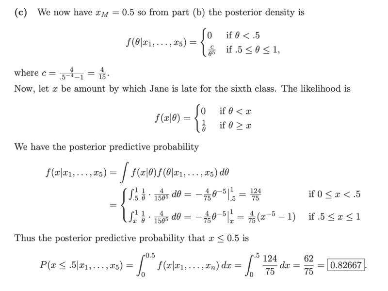
1. Where has this posterior predictive probability come from (see image for part(c) solution)? It vaguely seems like a marginalization integral to me, but am confused otherwise.
2. Why are there two separate integrals for the posterior predictive probability over the different ranges of ##x## (see image for part(c) solution, but requires a result from part (b))? Would someone be able to explain that to me please?

Context:
Part (a)
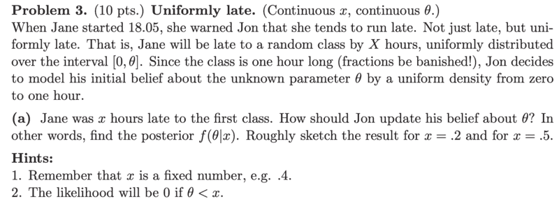
Screen Shot 2021-05-26 at 10.45.31 AM.png

Part(a) solution:

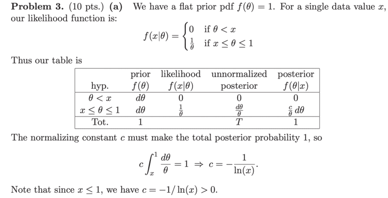
Screen Shot 2021-05-26 at 10.46.06 AM.png
Part (b):
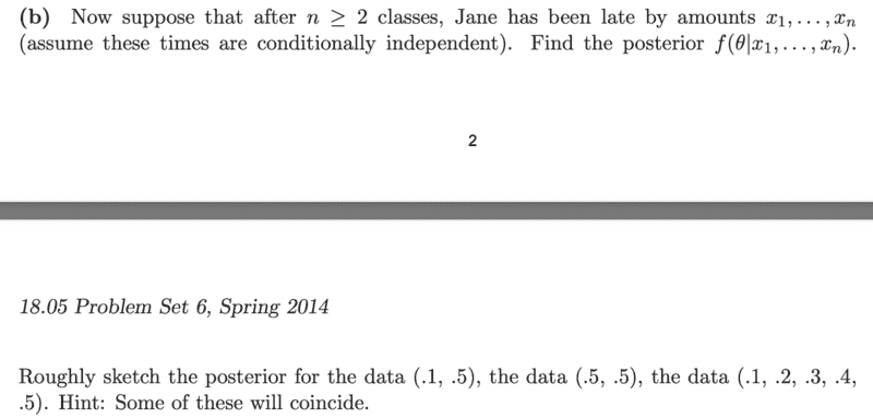
Screen Shot 2021-05-26 at 10.46.33 AM.png
Part (b) solution:
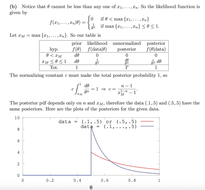
Screen Shot 2021-05-26 at 10.47.54 AM.png


Part (c):
Screen Shot 2021-05-26 at 10.47.19 AM.png


Part (c) solution: (this is what my question is about)
Screen Shot 2021-05-26 at 10.48.52 AM.png
Any help is greatly appreciated
 
Physics news on Phys.org
1) Yes, it is marginalisation. You know the probability given ##\theta## and you know the probability of each ##\theta##. The probability distribution for ##x## becomes the marginalised probability distribution. This is the continuous variable equivalent of ##P(A|B) = P(A|C) P(C|B) + P(A|\bar C) P(\bar C | B)## where ##C## and ##\bar C## are complementary.

2) There is one integral because you need to integrate the pdf for ##x## from 0 to 1/2. There is another integral arising from the fact that an integral appears in the marginalised probability.
 
Orodruin said:
1) Yes, it is marginalisation. You know the probability given ##\theta## and you know the probability of each ##\theta##. The probability distribution for ##x## becomes the marginalised probability distribution. This is the continuous variable equivalent of ##P(A|B) = P(A|C) P(C|B) + P(A|\bar C) P(\bar C | B)## where ##C## and ##\bar C## are complementary.

2) There is one integral because you need to integrate the pdf for ##x## from 0 to 1/2. There is another integral arising from the fact that an integral appears in the marginalised probability.
Thank you @Orodruin ! I will take some time to think about what you have written to internalize the content. However, just some initial follow up questions are:

With your answer to (2), I think that is starting make slightly more sense now. However, why has the solution provided an integral for the range ## 0.5 \leq x \leq 1 ##? It seems almost redundant to me...
 
Master1022 said:
With your answer to (2), I think that is starting make slightly more sense now. However, why has the solution provided an integral for the range 0.5≤x≤1? It seems almost redundant to me...
This is in the integral over ##\theta##. While the observation makes ##\theta > 1/2## less likely, it is still a possibility that you need to take into account.
 
Orodruin said:
This is in the integral over ##\theta##. While the observation makes ##\theta > 1/2## less likely, it is still a possibility that you need to take into account.
Thanks for your reply. I'm really sorry to ask, but is there perhaps another way you can explain it as I am still struggling to understand it.

So what I understand is:
1. We have our posterior density function from part (b)
2. Now we want to predict the likelihood of Jane being less than 0.5 hours late to next one
3. We form the likelihood just as in part (a)
4. We need to consider all the different scenarios of ##\theta## and integrate over them

Why do we split up the range into ## < 0.5 ## and ## 0.5 \leq x \leq 1 ##? I know the 0.5 is what part of the main question.

Is it because the likelihood cannot be non-zero when ##\theta < 0.5##. Therefore, ## theta ## is limited by ## min(x, 0.5) ## and 1? I am really sorry if this is worded poorly - I am finding it quite hard just to formulate exactly what I don't understand.
 
Yesterday I realized that 'posterior predictive distributions' was another concept in itself so I went away to watch some videos on it. I didn't know about it before and was just coming from a background of knowing about MLE and MAP
 
There are two things I don't understand about this problem. First, when finding the nth root of a number, there should in theory be n solutions. However, the formula produces n+1 roots. Here is how. The first root is simply ##\left(r\right)^{\left(\frac{1}{n}\right)}##. Then you multiply this first root by n additional expressions given by the formula, as you go through k=0,1,...n-1. So you end up with n+1 roots, which cannot be correct. Let me illustrate what I mean. For this...
Back
Top