Programming a Diffraction Pattern by the (pseudo?) method of images

39 replies · 7K views · last reply
PhDeezNutz
Messages
859
Reaction score
570
Homework Statement
I want to get a diffraction pattern from a circular hole in the Franhofer limit. In another thread I have been studying radiation patterns of various configurations and now I seek to study diffraction. I want to see if it's possible to place electric and magnetic dipoles in the vicinity of the hole and produce a respectable diffraction pattern on the far wall. The hole is in the XZ-plane and I want to graph the flux through a far away y = constant plane. I'm assuming normally incident plane wave through the hole.
Relevant Equations
From Jackson 9.16 we have the following equations for the vector potential of a radiating electric dipole and radiating magnetic dipole.

$$\vec{A} \left(\vec{r}\right) = - \frac{i \mu_0 \omega}{4 \pi} \left( \frac{e^{ikR}}{R}\right) \vec{p}$$

$$\vec{A} \left(\vec{r}\right) = \frac{\mu}{4 \pi} \left( \frac{e^{ikR}}{R^2} \right) \left( -ikR + 1\right)\vec{m} \times \vec{R}$$

(I don't think the last formula is in Jackson but I have used it to create a qualitatively accurate animation of a radiating magnetic dipole)

Naturally the ##\vec{B}## and ##\vec{E}## can be calculated by taking the curl and multiplying by the appropriate constant in the latter case.

$$\vec{B} = \nabla \times \vec{A}$$

$$\vec{E} = \frac{i}{k \sqrt{\mu \epsilon}} \nabla \times \vec{B}$$

The Poynting Vector field can then be found by taking the real parts of ##\vec{B}## and ##\vec{E}## and doing a cross product.

$$\vec{S} = \mathfrak{R} \left( \vec{E} \right) \times \mathfrak{R} \left( \vec{B}\right)$$
I oriented a magnetic dipole perpendicular to the hole (parallel to the ŷ ŷ y^ŷ direction) with one end at it's origin and I get the following pattern

3D surface plot in MATLAB style with x-axis from -1 to 1, z-axis from -1 to 1 and a y-axis labelled y-value scaled by 10^-12. The surface is dense with noisy spikes and has a circular dip near the centre.
I was really looking for something like this
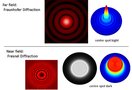
Comparison of diffraction patterns: top row labelled Far field Fraunhofer Diffraction shows concentric rings with a bright centre spot; bottom row labelled Near field Fresnel Diffraction shows rings with a dark centre spot, in 2D and 3D plots.


As you can see I'm getting almost the exact opposite of what I want since I'm going for Fraunhofer Diffraction. Conventional wisdom would suggest "if you want the exact opposite do the exact opposite". I have tried making the magnetic dipole parallel to the hole and I lose rotational symmetry in the flux symmetry on the back wall which is something I would not have expected.

I am open to suggestions and although I have tried many different combinations only to start back at square 1.

I would think I need to add more sources and separate them so as to have path length differences. Should they be electric dipoles or other magnetic dipoles.

I read Han's Bethe's paper "On the Theory of Diffraction by Small Holes" and the values he derived were

|p⃗ |=13π(a3)E0|p→|=13π(a3)E0​


and


|m[FONT=STIXGeneral-Regular]⃗ [FONT=STIXVariants]|[FONT=STIXGeneral-Regular]=23[FONT=STIXGeneral-Italic]π[FONT=STIXGeneral-Regular]([FONT=STIXGeneral-Italic]a[FONT=STIXGeneral-Regular]3)[FONT=STIXGeneral-Italic]H[FONT=STIXGeneral-Regular]0|m→|=23π(a3)H0​
I believe he oriented the electric field vector in the z-direction and the magnetic dipole in the y-direction. When I do such a configuration I do not remotely get a valid interference pattern on the back wall. I could have misinterpreted his paper. It was hard to read.

For the record I don't even know if my approach is valid.
 
  • Like
Likes   Reactions: kent davidge and JD_PM
3D surface plot of flux through a plane against x and z axes, showing a bright raised central peak with concentric ring ripples decaying outward over a dark blue background.


I believe I captured "Fresnel Diffraction" by putting a single electric dipole in the y-direction . Of course when I do this the radiation flux disappears on the axis making it pretty much impossible to get a central maxima (what I was hoping for with "Fraunhofer" diffraction).

Then again maybe when I take a closer look at my program I will find the choices of wavelengths and distances do not conform to that limit. I'll take a look at it after dinner.

Maybe I trivially plotted the flux pattern of a single electric dipole and it resembles Fresnel Diffraction by mere coincidence.

Edit: In my opinion Jackson's explanation of Fresnel vs. Fraunhofer diffraction is kind of confusing.
 
Last edited:
  • Like
Likes   Reactions: kent davidge
you say in the OP
PhDeezNutz said:
I want to get a diffraction pattern from a circular hole in the Franhofer limit

why not consider an incident plane wave? would simplify things considerably..

maybe you are looking for something more realistic?
 
PhDeezNutz said:
I was really looking for something like this
those patterns are obtained when a plane wave hits the aperture
 
kent davidge said:
you say in the OPwhy not consider an incident plane wave? would simplify things considerably..

maybe you are looking for something more realistic?

Although it's not in my code I believe I am considering an incident plane wave on the aperture with a circular opening. I'm basically trying to place a secondary source in the vicinity of the aperture that would mimic how the plane wave changes.Are you saying I should add back the plane wave to the wave I have? I could try that. I think I'd have to create a dipole far away from the aperture that would result in plane wave front near the aperture. Should I make that dipole big or small in magnitude compared to the dipole I have near the aperture?
 
PhDeezNutz said:
mimic how the plane wave changes
ah, that's the problem. your software requires that you manually produce waves beyond the hole as if they were a result of the original wave being diffracted

this being the case, then...
PhDeezNutz said:
I think I'd have to create a dipole far away from the aperture that would result in plane wave front near the aperture. Should I make that dipole big or small in magnitude compared to the dipole I have near the aperture?
I think the best way you can do it is by creating a large number* of spherical waves emanating from different points on the aperture, since that's how the diffracted waves can be expressed (it is known as the Huygens' principle)

*you actually need an infinite number of them to satisfy the Huygens' principle, but if you don't have a manageable way of including infinities in your software, then a large number of them would presumably give a good approximation.
 
  • Like
Likes   Reactions: PhDeezNutz
I can only program radiating dipoles, quadrupoles, and sometimes octupoles. Starting with the most elementary case should I fill the hole with a bunch of tiny dipoles in a outwardly radial pattern?
 
You should fill the hole in the XZ plane with dipoles (all aligned) radiating radially outward (towards your target). The sum over the circle should give you the appropriate Bessel-ish function at target.
 
  • Like
Likes   Reactions: PhDeezNutz
hutchphd said:
You should fill the hole in the XZ plane with dipoles (all aligned) radiating radially outward (towards your target). The sum over the circle should give you the appropriate Bessel-ish function at target.

I don't quite understand. How can they all be aligned and pointing radially outward? And if they are radially outward how can they be pointing towards the target (the wall?).

Maybe I'm just having a brain fart.
 
You have the geometry wrong. The p will point in the polarization direction of the incident plane wave...choose that to be the z axis. Why are you including both a magnetic dipole and an electric one? i think you want to just do an array of electric dipoles in th xy plane at least to start.
 
  • Like
Likes   Reactions: PhDeezNutz
So I've been doing some reading and looking around and indeed according to the book "Applied Scanning Probe Methods II: Scanning Probe Microscopy Techniques" (Novotny and Hecht)

and the supposed far field diffraction pattern of circular aperture can be reproduced by this substitute arrangement (According to Bethe and Bouwkamp).

Fig. 10.5 diagram: far-field emission of a subwavelength aperture modeled as an electric dipole Peff along the axis and a magnetic dipole Meff in the screen plane, with |E|^2=cos θ and |H|^2=cos θ lobes shown as dashed curves.


To me this is insane. I don't see how you can get a central maxima in this configuration because to my understanding radiation disappears on the axis of the dipoles (in this case ##\vec{p}##).

I have used my programs to produce a qualitatively accurate pattern of both kinds of dipoles. I combined them and I am getting the following

3D surface plot in MATLAB style of flux through a plane parallel to the xz-plane, showing a central peak near 10 x 10^5 with concentric ringed ripples decaying outward over x and z axes from -3000 to 3000.


Pretty much the same as my last one. This time with supported literature (that doesn't seem feasible to me).
 
How big is wavelength for graph?
Units on axes are ?
 
  • Like
Likes   Reactions: PhDeezNutz
I set the radius of the circle equal to


a=1a=1​
and


k=5π1000⇒λ=2πk=400k=5π1000⇒λ=2πk=400​
I think that conforms to the long wave-length limit.

I cut the figure with the

y=460yy=460y​

plane. Perhaps I should do it over 10 to 100 wavelengths?

Edit: The units on the vertical axis is Poynting Flux of the y-component of the Poynting Vector. (I don't know the units for the Poynting Vector of the top of my head).
 
I'm so sorry for the Latex messing up. The aperture has a radius of 1. The wavelength is 400. I cut with the y = 460 plane.

The units on the vertical axis is poynting flux through the plane. I.e. the y-component of the poynting vector.
 
A good test of your calculation might be to cut the wave length to 40 (factor of 10) and see how stuff scales. Just do one thing at a time!
 
  • Like
Likes   Reactions: PhDeezNutz
hutchphd said:
A good test of your calculation might be to cut the wave length to 40 (factor of 10) and see how stuff scales. Just do one thing at a time!

I cut it down to 40 and for some reason I lost cylindrical symmetry. That doesn't make sense to me.
3D surface plot in MATLAB style: flux through arbitrary plane parallel to xz-plane (times 10^5) against x-axis and z-axis, with a tall central peak near x = 500 to 1000 reaching about 5 x 10^5, surrounded by a noisy, rippled surface with negative dips down to about -2 x 10^5.

Heatmap plot of a square grid with x-axis and z-axis ticks from -2500 to 2500, showing a bright yellow-green square-ring pattern near the centre and dimmer blue arcs spreading outward.


It's just hard for me to imagine there being radiation on a dipole axis.
 
PhDeezNutz said:
I cut it down to 40 and for some reason I lost cylindrical symmetry. That doesn't make sense to me
I'm flying blind here...the only square in the problem is your calculation mesh (?) ...is that showing up in the result suddenly (?) . Well I'm shot for the eve...
 
hutchphd said:
I'm flying blind here...the only square in the problem is your calculation mesh (?) ...is that showing up in the result suddenly (?) . Well I'm shot for the eve...

It seems to be the case. I’m not sure.

Do you agree that that radiation disappears on the axis of the dipoles? Every picture I’ve seen of dipole radiation has this “donut” feature.

Thanks for your help btw. We’ll figure this out hopefully.
 
Glad to try to help. Actually did enough reading to know I was woefully ignorant about exactly what this was about. So here is an interesting paper I found which seems good but whose exact provenance I couldn't decipher:

https://www.photonics.ethz.ch/fileadmin/user_upload/Courses/NanoOptics/ProjectReports/aperture.pdf

Sooo...this is more involved than I understood. Check out the paper and I need to understand exactly what you wish to see.
 
  • Like
Likes   Reactions: PhDeezNutz
hutchphd said:
Glad to try to help. Actually did enough reading to know I was woefully ignorant about exactly what this was about. So here is an interesting paper I found which seems good but whose exact provenance I couldn't decipher:

https://www.photonics.ethz.ch/fileadmin/user_upload/Courses/NanoOptics/ProjectReports/aperture.pdf

Sooo...this is more involved than I understood. Check out the paper and I need to understand exactly what you wish to see.

Will do and this paper looks promising. I don't think you were woefully ignorant. As you said the dipoles should be in the z-direction.

I actually thought about making a spherical shell of uniformly oriented dipoles but was hesitant to because of how hard it would be (for me) to write the program so I desperately tried a bunch of random configurations to no avail.

At first glance, the sphere/ spherical shell should produce a spherical wavefront at the back wall and give us the desired Bessel function profile.

Thanks again, looks like I have my work cut out for me. Have to work on my numerical integration.
 
  • Like
Likes   Reactions: hutchphd
3D surface plot in MATLAB style of flux through an arbitrary plane parallel to the xz-plane, with a noisy, jagged surface colored in teal, green and yellow, spiking near the centre and dipping below zero, axes in units of 10^6 and 10^-69.


Strange to say the least. I'm going to try and pointing the vector radially at each point in the sphere. I'm afraid I'll get vanishing radiation everywhere but it doesn't hurt to try.
 
3D surface plot in MATLAB style, flux through a plane parallel to the xz-plane, with z-axis from -1 to 1 and x-axis from -1 to 1 (times 10^6), jagged mesh with multicoloured faces and a vertical scale of about -2 to 2 times 10^-59.


Not getting any better. If I programmed that right then that is not what I'm looking for.
 
Should the flux be negative? Actually can it be negative if your calculation is working?
 
  • Like
Likes   Reactions: PhDeezNutz
hutchphd said:
Should the flux be negative? Actually can it be negative if your calculation is working?

That is a very good point. You are right, it should not be negative. I’ll look over my program again.
 
3D surface plot in MATLAB-style colours of flux through a plane parallel to the xz-plane, with x-axis from -3000 to 3000 and z-axis from -3000 to 3000, showing a central peak with ripples decaying outward.


This is the best I've gotten. Again this is flux through a ##y = constant## plane. I got this by putting a dipole at the origin and pointing it in the ##\vec{p_1} = (0,1,2)## direction. My first thought was to put another dipole at the origin and point it in the ##\vec{p_2} = (0,1,-2)## direction to bring up the other side of the envelope and accentuate the peak but that just gives us a dipole pointing along the y-axis (i.e. cylindrically symmetric flux pattern but no central peak as before).

Instead what I'm going to do is put ##\vec{p_2} = (0,1,-2)## on the ##y-axis## far away from the origin. Hopefully that will bring up the envelope on the other side, accentuate the peak, and not cancel out (because ##\vec{p_2}## is so far away from ##\vec{p_1}##.

When I extend the scale of the problem at the beginning of this post to ##\approx 10## times I start losing the central peak. When I extend the scale of the problem at the beginning of this post ##\approx 100## times I start getting negative flux. The only thing I changed was the extend of the grid, nothing else and I'm getting very weird results.

3D surface plot in MATLAB style of flux through a plane parallel to the xz-plane, with x-axis and z-axis scaled by 10^4 and flux values up to 2.5 x 10^-11; the surface shows a central peak with ripple artifacts across the grid.


3D surface plot in MATLAB style of flux through a plane parallel to the xz-plane, showing a rough, spiky surface with peaks up to about 4 x 10^-16 and dips to about -3 x 10^-16 over x and z axes of +/-1 x 10^5.


I also tried taking the sphere of dipoles and shrinking by a factor of 100 in hopes of getting rid of the negative flux to no avail.
 
I made ##\vec{p_1} = (0,1,2)## @ ##(0,0,0)## and ##\vec{p_2} = \frac{1}{10} (0,-1,2)## @ ##(0,-constant,0)## where the constant is far away from the diffracting aperture.

Getting more coverage with the envelope while maintaining the peak. If I deviate from multiplicative magnitude constant ##\frac{1}{10}## I start to lose desirable features.

Still not getting full coverage though. I might sound crazy but I really think going forward the strategy is to move away from the aperture on the incident side and start introducing electric and magnetic dipoles in that region. It has gotten me the best result thus far albeit not perfect.
3D surface plot of flux through an arbitrary plane parallel to the xz-plane, with z-axis ranging from -2000 to 2000, x-axis from -2500 to 2500, and flux scaled by 10^-10 from -0.5 to 4.5, showing a central peak with ripple-like oscillations.

Color-mapped plot of concentric ring interference fringes over x-axis and z-axis from -2500 to 2500, with a bright yellow central spot at the origin fading to dark blue at the edges.
 
Last edited:
Nvm I programmed my separation vectors from the two dipoles wrong. The picture above is therefore not valid.
 
3D surface plot in MATLAB style, flux through arbitrary plane parallel to xz-plane, z-axis in units of 10^-4, showing a dome-shaped surface with values mostly negative from about -14 to 0 across x from -2500 to 2500.


I used the method of images for a dipole inside a circle. I made the radius of the circle equal to the distance from the aperture plane to the projecting plane and made the distance from the origin to the dipole arbitrary (but less than the aforementioned distance). Don't know why it's negative.
 
I think if I can correctly combine the following flux patterns I will get a Bessel function type flux pattern.

3D surface plot in MATLAB style of flux through a plane parallel to the xz-plane, plotted over x-axis and z-axis from -3000 to 3000, with a central raised circular peak and concentric ripples that decay outward.


3D surface plot of flux through an arbitrary plane parallel to the xz-plane, plotted against x-axis from -2500 to 2500 and z-axis from -2000 to 2000, with a single smooth arched surface peaking near the center and colored by value from blue at the edges to yellow-orange at the top.
 
Please disregard the last post. I took a second look at my program and I put my dipoles in the wrong places according to the method of images configuration of a dipole in a sphere. I re-programmed it and my result is the following (first picture). I believe if I can correctly combine it with the second picture I will get my desired Bessel Function.
3D surface plot of flux through an arbitrary plane parallel to the xz-plane, with z-axis and x-axis from -3000 to 3000 and flux values from -0.15 to 0, showing a central peak surrounded by concentric ring-like oscillations.


3D surface plot in MATLAB style of flux through an arbitrary plane parallel to the xz-plane over x-axis and z-axis from -3000 to 3000, showing a raised central peak with concentric ripples falling off outward.


Combining them without compromising the desirable features of either graph might prove difficult. I am happy with the central peak in the first picture despite it not being significantly higher than the ridges around it.