babaliaris
- 117
- 15
- TL;DR
- Replicating Wang-Haiting space-charge field equations results in 4.2 kV/cm peak (Instead of 5) despite maxing parameters. Seeking insights on potential integration or normalization discrepancies.
Hello guys!
I'm a senior electrical & computer engineer at Aristotle University of Thessaloniki (Greece), and I'm working on my Thesis: A Software Application For Simulating the Effects of Space Charge In A Rod-Plane Gap, which depends heavily on the work of Wang Wenduan, Wang Haiting (source paper is provided in the attachments).
In the attachments, I provided my entire proof of the field equations (the document is written in the LyX editor) that includes mathematical alignment with Wang Wenduan, Wang Haiting math framework. You can find the python code I used to achieve the numerical calculations: https://github.com/babaliaris/space-charge-sim.
Please note that this is my very first experience with solving numerical problems in a real problem. I never attempted solving something that can not be solved analytically (exams, exercises, etc). So I pretty much have no clue what I have to do or what test/experiments to execute. I follow some instructions I got from my Professor.
These are my results:
Space Charge Density Function (Given by Wang Wenduan, Wang Haiting):
$$
\rho(r)=\frac{A}{\left(r+C\right)^{B}}\;\;\left[\frac{C}{m^{3}}\right]\;\;,\;\;\text{Domains:}\begin{cases}r\in\left[0\;,\;L_{cs}\right]\\\theta\in\left[0\;,\;\theta_{B}/2\right]\\\phi\in[0\;,\;2\pi]\end{cases}
$$
A Parameter (B and C are chosen such that the total field, including the applied external/geometric field, becomes constant / uniform):
$$
A(\;E_{c}\;,\;B\;,\;C\;,\;L_{cs}\;,\;\theta_{B}\;)=\frac{\overbrace{\pi\epsilon_{0}E_{c}L^{2}_{cs}\tan^{2}\left(\frac{\theta_{B}}{2}\right)}^{Q_{cs}}}{2\pi\left[1-\cos\left(\frac{\theta_{B}}{2}\right)\right]\int^{L_{cs}}_{0}\frac{r^{2}}{(r+C)^{B}}\,dr}$$
Space Charge Attenuation Distance:
$$
r_{1}=\sqrt{\left[z-R-rcos(\theta)\right]{}^{2}+\left[rsin(\theta)\right]^{2}}
$$
Space Charge Electric Field:
$$
\vec{E}_{sp}=\frac{1}{2\epsilon_{r}\epsilon_{0}}\int^{\frac{\theta_{B}}{2}}_{0}\int^{L_{cs}}_{0}\frac{\rho(r)r^{2}sin(\theta)}{r^{3}_{1}}[z-R-rcos(\theta)]drd\theta\hat{z}
$$
Distance Between Space Charge And Rod (espherical-electrode) Center:
$$
r_{2}=\sqrt{\left[R+rcos(\theta)\right]^{2}+\left[rsin(\theta)\right]^{2}}
$$
Distance Of The Rod Image Charge From The Center Of The Spherical Rod (Sir William Thomson, Lord Kelvin):
$$
r_{3}=\frac{R^{2}}{r_{2}}
$$
Rod Image Charge Attenuation Distance:
$$
r_{4}=\sqrt{\left(z-\frac{r_{3}}{r_{2}}\left[R+rcos(\theta)\right]\right)^{2}+\left(\frac{r_{3}}{r_{2}}rsin(\theta)\right)^{2}}
$$
Rod Image Electric Field:
$$
\vec{E}_{I_{rod}}=-\frac{1}{2\epsilon_{r}\epsilon_{0}}\int^{\frac{\theta_{B}}{2}}_{0}\int^{L_{cs}}_{0}\frac{\rho(r)r^{2}Rsin(\theta)}{r^{3}_{4}r_{2}}\left[z-\frac{r_{3}}{r_{2}}\left(R+rcos(\theta)\right)\right]drd\theta\hat{z}
$$
Plane Image Charge Attenuation Distance:
$$
r_{5}=\sqrt{\left[rsin(\theta)\right]^{2}+\left(2d-rcos(\theta)-R-z\right)^{2}}
$$
Plane Image Charge Electric Field:
$$
\vec{E}_{I_{plane}}=\frac{1}{2\epsilon_{r}\epsilon_{0}}\int^{\frac{\theta_{B}}{2}}_{0}\int^{L_{cs}}_{0}\frac{\rho(r)r^{2}sin(\theta)}{r^{3}_{5}}\left(2d-rcos(\theta)-R-z\right)drd\theta\hat{z}
$$
By the way, I have extended the framework to include the image contribution of the grounded plane, something that Wang Wenduan, Wang Haiting did not include, since they only studied what is going on very close to the rod-electrode (and away from the plane, meaning Eplane = 0). In my following results, I did the same.
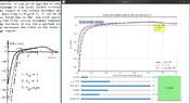
Currently, I'm trying to replicate their Figure 3: Electric field distribution in the vicinity of the rod tip owing to space charge. However, they do not provide what parameters they used for A, B, C, and θB (they tell you how to choose them). The idea is to select B and C such that:
$$E_{ext} + E_sp + E_{I} = constant$$
since the experiments showed that the total field becomes uniform and almost constant, even though the space charge field is extremely non-uniform.
In their results, they do not show how they calculated Eext (external, voltage applied to the electrode); they do, however, mention the method and have a source for it.
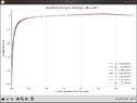
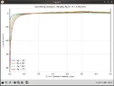
The problem is, that in my results I had to max the parameters for θB=80 degrees and Ec=7kV/cm to reach close to their data, which is probably wrong because they say they used Ec=5kV/cm.
I do not know what to do next.
Thank you for your time.
I'm a senior electrical & computer engineer at Aristotle University of Thessaloniki (Greece), and I'm working on my Thesis: A Software Application For Simulating the Effects of Space Charge In A Rod-Plane Gap, which depends heavily on the work of Wang Wenduan, Wang Haiting (source paper is provided in the attachments).
In the attachments, I provided my entire proof of the field equations (the document is written in the LyX editor) that includes mathematical alignment with Wang Wenduan, Wang Haiting math framework. You can find the python code I used to achieve the numerical calculations: https://github.com/babaliaris/space-charge-sim.
Please note that this is my very first experience with solving numerical problems in a real problem. I never attempted solving something that can not be solved analytically (exams, exercises, etc). So I pretty much have no clue what I have to do or what test/experiments to execute. I follow some instructions I got from my Professor.
These are my results:
Space Charge Density Function (Given by Wang Wenduan, Wang Haiting):
$$
\rho(r)=\frac{A}{\left(r+C\right)^{B}}\;\;\left[\frac{C}{m^{3}}\right]\;\;,\;\;\text{Domains:}\begin{cases}r\in\left[0\;,\;L_{cs}\right]\\\theta\in\left[0\;,\;\theta_{B}/2\right]\\\phi\in[0\;,\;2\pi]\end{cases}
$$
A Parameter (B and C are chosen such that the total field, including the applied external/geometric field, becomes constant / uniform):
$$
A(\;E_{c}\;,\;B\;,\;C\;,\;L_{cs}\;,\;\theta_{B}\;)=\frac{\overbrace{\pi\epsilon_{0}E_{c}L^{2}_{cs}\tan^{2}\left(\frac{\theta_{B}}{2}\right)}^{Q_{cs}}}{2\pi\left[1-\cos\left(\frac{\theta_{B}}{2}\right)\right]\int^{L_{cs}}_{0}\frac{r^{2}}{(r+C)^{B}}\,dr}$$
Coordinate Systems & Reference Frames
When implementing these equations, note that the calculations bridge two different coordinate frames:- Global Coordinate System (z): Origin at the center of the rod-electrode, with the observer coordinate z measured directly from this global center.
- Local Coordinate System (r, θ, θB, Lcs): Centered at the cone apex (tip) of the charge distribution geometry, which is located at
$$ (0,0,R) = R\hat{z}$$ in global coordinates, where R is the radius of the rod. Wang Wenduan & Wang Haiting have their origin at the conical apex (tip), this means that if Zwh is their observation point, my observation point can be related linearly using the coordinate transformation:
$$Z = Zwh + R$$
Space Charge Attenuation Distance:
$$
r_{1}=\sqrt{\left[z-R-rcos(\theta)\right]{}^{2}+\left[rsin(\theta)\right]^{2}}
$$
Space Charge Electric Field:
$$
\vec{E}_{sp}=\frac{1}{2\epsilon_{r}\epsilon_{0}}\int^{\frac{\theta_{B}}{2}}_{0}\int^{L_{cs}}_{0}\frac{\rho(r)r^{2}sin(\theta)}{r^{3}_{1}}[z-R-rcos(\theta)]drd\theta\hat{z}
$$
Distance Between Space Charge And Rod (espherical-electrode) Center:
$$
r_{2}=\sqrt{\left[R+rcos(\theta)\right]^{2}+\left[rsin(\theta)\right]^{2}}
$$
Distance Of The Rod Image Charge From The Center Of The Spherical Rod (Sir William Thomson, Lord Kelvin):
$$
r_{3}=\frac{R^{2}}{r_{2}}
$$
Rod Image Charge Attenuation Distance:
$$
r_{4}=\sqrt{\left(z-\frac{r_{3}}{r_{2}}\left[R+rcos(\theta)\right]\right)^{2}+\left(\frac{r_{3}}{r_{2}}rsin(\theta)\right)^{2}}
$$
Rod Image Electric Field:
$$
\vec{E}_{I_{rod}}=-\frac{1}{2\epsilon_{r}\epsilon_{0}}\int^{\frac{\theta_{B}}{2}}_{0}\int^{L_{cs}}_{0}\frac{\rho(r)r^{2}Rsin(\theta)}{r^{3}_{4}r_{2}}\left[z-\frac{r_{3}}{r_{2}}\left(R+rcos(\theta)\right)\right]drd\theta\hat{z}
$$
Plane Image Charge Attenuation Distance:
$$
r_{5}=\sqrt{\left[rsin(\theta)\right]^{2}+\left(2d-rcos(\theta)-R-z\right)^{2}}
$$
Plane Image Charge Electric Field:
$$
\vec{E}_{I_{plane}}=\frac{1}{2\epsilon_{r}\epsilon_{0}}\int^{\frac{\theta_{B}}{2}}_{0}\int^{L_{cs}}_{0}\frac{\rho(r)r^{2}sin(\theta)}{r^{3}_{5}}\left(2d-rcos(\theta)-R-z\right)drd\theta\hat{z}
$$
By the way, I have extended the framework to include the image contribution of the grounded plane, something that Wang Wenduan, Wang Haiting did not include, since they only studied what is going on very close to the rod-electrode (and away from the plane, meaning Eplane = 0). In my following results, I did the same.
Currently, I'm trying to replicate their Figure 3: Electric field distribution in the vicinity of the rod tip owing to space charge. However, they do not provide what parameters they used for A, B, C, and θB (they tell you how to choose them). The idea is to select B and C such that:
$$E_{ext} + E_sp + E_{I} = constant$$
since the experiments showed that the total field becomes uniform and almost constant, even though the space charge field is extremely non-uniform.
In their results, they do not show how they calculated Eext (external, voltage applied to the electrode); they do, however, mention the method and have a source for it.
The problem is, that in my results I had to max the parameters for θB=80 degrees and Ec=7kV/cm to reach close to their data, which is probably wrong because they say they used Ec=5kV/cm.
I do not know what to do next.
Thank you for your time.
Attachments
-
A Software Application For Simulating The Effects Of Space Charge In A Rod-Plane Gap.pdf888.2 KB · Views: 9
-
 peak_result.webp78.4 KB · Views: 13
 -
 varying_Ec.webp31.2 KB · Views: 13
 -
 varying_thetaB.webp30.3 KB · Views: 11
 -
a-new-model-for-simulating-the-effects-of-space-charge-in-gas-di.pdf298.4 KB · Views: 13
