Simulink: designing a 2nd order sliding controller

Click For Summary
SUMMARY

This discussion focuses on designing a second-order sliding mode controller (SMC) using Simulink for a slip control problem. The user has derived a differential equation for slip dynamics but lacks a transfer function for implementation. The recommended approach is to represent the dynamics using signal networks in Simulink, utilizing integration blocks to solve the differential equation directly. Tools within Simulink, such as Bode plots, can assist in analyzing the system without requiring a known transfer function.

PREREQUISITES
  • Understanding of differential equations and their applications in control systems.
  • Familiarity with Simulink for modeling and simulation.
  • Knowledge of sliding mode control principles and their implementation.
  • Basic concepts of signal processing, including summation and multiplication of signals.
NEXT STEPS
  • Learn how to implement differential equations in Simulink using integration blocks.
  • Explore the use of Bode plots in Simulink for system analysis.
  • Study the principles of sliding mode control in depth to enhance controller design.
  • Investigate methods for estimating parameters in dynamic systems without known transfer functions.
USEFUL FOR

Control engineers, systems modelers, and researchers focusing on advanced control strategies and simulation techniques in MATLAB and Simulink.

Payam30
Messages
44
Reaction score
1
Hi,
I've had obtained a mathematical model for the slip controller issue.
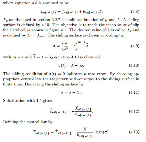
cwyNyiR.png

As you see I have the diffequation for the slip. and the input that force the system to zero error is provided as well. Now it's time to implement it in simulink or matlab.
I took a look at the example provided on mathwork. Here is a screen shot
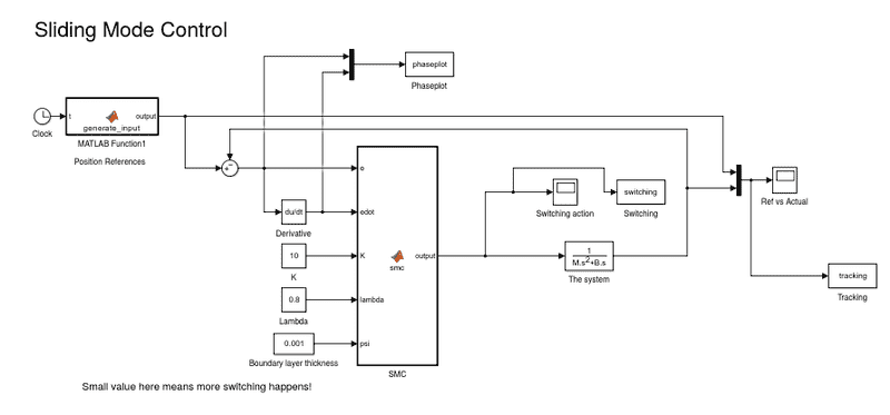
SXq2FER.png

The controller is supposed to force \lambda to a certain value. The optimal input is provided as well. So the reference block should be \lambda_desired. That's correct and then it goes to SMC and it gives the input to the system. What is that system? is it the dynamics of the slip? I have only the dynamics in mathematical way and no transfer function. You see that the dynamics of the slip is:
ZQTA0Lg.png

where T is the input . g is constant. R supposed to be observed by a observer. \lambda is slip and J is inertia. \mu is friction and assumed to be constant. \omega is the rotational speed on the wheel. How do I convert this to transfer function. I really need help since I ve done a lot and stuck in this. Please help me with this.
 
Physics news on Phys.org
I don't understand a lot of the specifics of your problem, but I have a general comment:
In many applications of Simulink, you do not know the transfer functions of some of the physics and they would be tremendously complicated. You use a Simulink diagram to implement the equations for the dynamics of the slip and run simulations to get results. There are tools to obtain Bode plots and estimate parameters.
 
Last edited:
Thank you for your response.
As you see in the picture, the input should go to the dynamic. The dynamic of the slip is :
## \dot{\lambda} = (- \frac{g}{R\omega} + \frac{Rmg(\lambda -1)}{\omega J})\mu - \frac{(\lambda -1)}{\omega J}T##
So this is the case:
Reference value ---> SMC -----> dynamics --->output
the output will get feedback to the SMC. My question is. I don't have any transfer function of the dynamics so how do I do this? how to I implement the dynamics in simulink
 
That equation for ##\dot{\lambda}## can be represented as a signal network with blocks for signal summing, multiplication, inversion, etc. Feed the result of that network into an integration block to obtain ##\lambda## and use that signal in the network as needed.
 
You mean that I should solve the differential equation instead of using the transfer funktion? That could work...
 
Yes. Simulink is used in a great number of simulations where the transfer function is not known but the equations can be represented in signal networks. It provides tools that can be used to analyse the system (Bode plots, etc.)
 
You were right. I did following scheme:
Lo11xdN.jpg

The SMC is as following:
u = u_d - \frac{K}{b} sat(\frac{\sigma}{\theta})
I have actually problem with founding \theta. This is the boundary thickness. anyone with insights in SMC.
 
Solved. Thanks
 

Similar threads

  • · Replies 11 ·
Replies
11
Views
4K
  • · Replies 0 ·
Replies
0
Views
2K
  • · Replies 0 ·
Replies
0
Views
2K
  • · Replies 1 ·
Replies
1
Views
4K
  • · Replies 5 ·
Replies
5
Views
5K
Replies
2
Views
8K
Replies
2
Views
3K
  • · Replies 1 ·
Replies
1
Views
2K
Replies
1
Views
2K
  • · Replies 4 ·
Replies
4
Views
22K