Solve Inaccurate CFD Predictions: Improve Results

[Smushiehippo]

Homework Statement

Find areas of potential inaccurate predictions in the simulation and improvements.

Relevant Equations

none

Hi
Im confused with what the CFD Results show or mean. I have never done CFD before and don’t have any material explaining it.
Question

Find areas of potential inaccurate predictions in the simulation and improvments.

This is the instructions I had to follow.
https://help.sim-flow.com/documentation/panels/hex-meshing
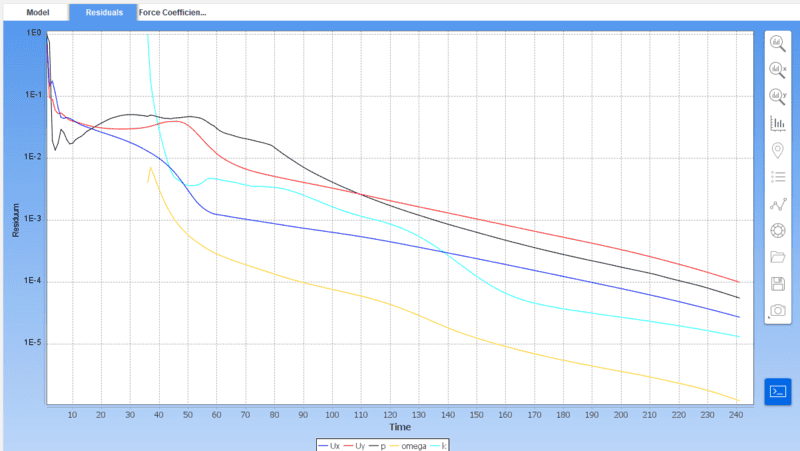
1st fig, The residuel graph, im not sure what this means or shows
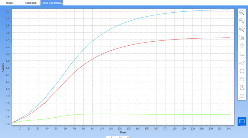
2nd fig, Coefficient, I think it it shows the 3 coefficient of lift, drag and pitch and time it takes to converge (but I don’t know what this means)
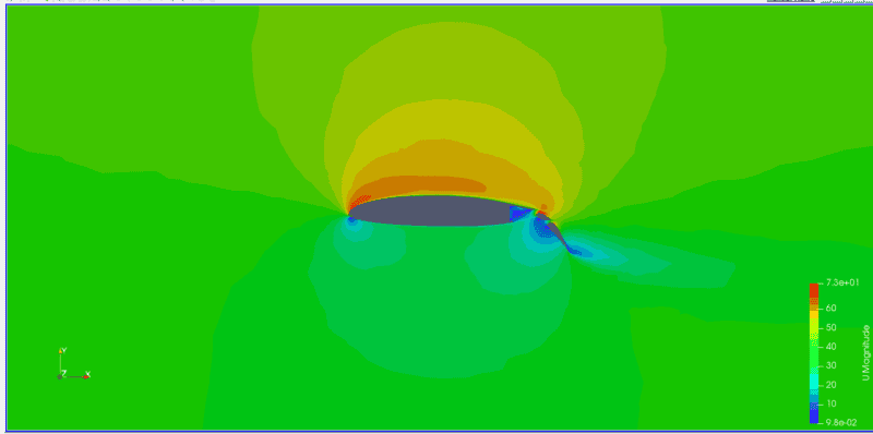
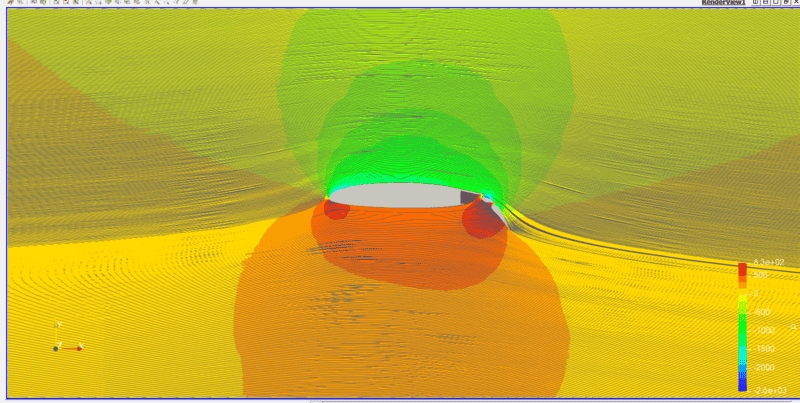
3rd and 4th, This velocity and pressure flow. High velcoity on top and low below. This indicates high pressure below and low pressure above generating lift. Increasing the velocity on top and decrease below would iMaxiumizing and mininzing the pressure producing improved lift.

Im try to extract information from it, understand it, but dont undestand what im looking at.
eg what are the residuals and what is it showing?

 

[bigfooted]

There is a nice series of youtube videos called cfd101 which covers many topics:
https://www.youtube.com/@fluidmechanics101/videos
For instance this one about residuals:


In short:
1st fig:
you are basically solving the system of equations Ax=b (A a matrix, x,b vectors) for the unknown x, which is the vector containing the solution of all variables, so pressure,velocity, etc at all points in the domain. During the iterations, you update your current estimate of the solution x. If you have the exact solution x, then Ax-b=0. As long as you do not have the exact solution, then Ax-b = R, with R a nonzero 'residual' vector. The residual plot shows for all variables the residual value. These residual values should be very low, 1e-4 is usually on the high side.
2nd fig:
During the iterations, you can compute values of lift, drag etc. It is not clear exactly what is shown in the figure, but you can see that the values seem to converge to a certain value. You can also see that they are still changing a little, so 240 iterations is not sufficient.

 

[Smushiehippo]

There is a nice series of youtube videos called cfd101 which covers many topics:
https://www.youtube.com/@fluidmechanics101/videos
For instance this one about residuals:


In short:
1st fig:
you are basically solving the system of equations Ax=b (A a matrix, x,b vectors) for the unknown x, which is the vector containing the solution of all variables, so pressure,velocity, etc at all points in the domain. During the iterations, you update your current estimate of the solution x. If you have the exact solution x, then Ax-b=0. As long as you do not have the exact solution, then Ax-b = R, with R a nonzero 'residual' vector. The residual plot shows for all variables the residual value. These residual values should be very low, 1e-4 is usually on the high side.
2nd fig:
During the iterations, you can compute values of lift, drag etc. It is not clear exactly what is shown in the figure, but you can see that the values seem to converge to a certain value. You can also see that they are still changing a little, so 240 iterations is not sufficient.

Just check i understood this right.

Fig.1 (residual graph) it solving various residuals, residuals being various properity of the object under study (pressure on the wing, velocity of the wing). It is done in iteractions. each iteraction it gets closer to zero, with zero being exact solution for the equation. as it gets closer to zero accuracy increases. high residual low accuracy, low residual high accuracy of the solutions. Solutions being the condions on the wing (pressure velocity and so on).
Fig.2 (force coefficient graph) it calculates the values of the 3 coeffcients (drag, lift and pitch). these values being the quantity of each it generates. when they converge they obtain more accurate value. so for this you would want drag line to be and lift line to be high.
fig.3 (velocity map), this shows the velocity and quantity over the wing and the pressure.
fig.4 (streamlines), this shows only the directions of the pressure flow.

for fig.4 why is it red underneath and not on top like in fig.3 like they flipped.

 

[bigfooted]

Yes, that's about right. I guess with iteractions you mean iterations? You can see the residuals as a measure for the error. For figure 2, the results do not need to be high, the lift and drag need to go to a value that does not change anymore with increasing iterations. This is an indication that you have reached your final solution.
in Fig 3,4, the red regions just indicate regions where the value is high. Velocity is high above the wing, pressure is high below the wing. If you follow a streamline, then Bernoulli's law tells you that when the velocity over a streamline increases, pressure decreases.