SUMMARY
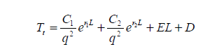
The discussion centers on creating a temperature profile function T(L) based on depth L, which varies from 0 to 500. User mk747pe inquired about plotting this function, and another participant confirmed that T(L) is already defined and can be graphed by substituting numerical values for constants. The example provided involved using constants of $1$ and $-1$ to demonstrate how to visualize the function effectively. The inquiry was resolved satisfactorily, confirming the user's understanding and needs.
PREREQUISITES
- Understanding of mathematical functions and graphing techniques
- Familiarity with the concept of temperature profiles in scientific contexts
- Basic knowledge of variable manipulation in equations
- Experience with graphing software or tools for visualizing functions
NEXT STEPS
- Explore graphing tools such as Desmos or GeoGebra for visualizing mathematical functions
- Learn about temperature profile modeling in environmental science
- Investigate how to manipulate and analyze functions in Python using libraries like Matplotlib
- Study the implications of different constants in temperature equations and their effects on graph shape
USEFUL FOR
Students, researchers, and professionals in environmental science, mathematics, and engineering who are interested in modeling and visualizing temperature profiles based on depth.