Understanding the heat equation solution derived in this article

[Makadamij]

Homework Statement

Try to understand the solving method of the three heat equations given in the following article.

Relevant Equations

1-dimensional heat equations - see the pictures below, please:

Hello everyone!

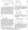
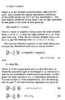
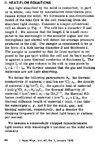
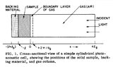
I'm analysing a scientific paper regarding the theory of the photoacoustic effect. The subject of investigation is a so called photoacoustic cell, in which a higly light-absorbing solid material is placed on a backing material and the rest of the cell is filled with gas (see picture below). Only the solid material is capable of absorbing light and converting it into heat. The cell is illuminated by sinosoidal chopped monochromatic light flux. The goal is to find the settled temperature distribution inside the cell. Therefore, three heat equations have been set up in picture pg65_2, two homogenous ones for the backing material and the gas and a non homogeneous heat equation for the solid, because heat is being created inside of it because of light absorption. The general solutions to these three equations are in picture pg66_1, not taking into account the boundary conditions of heat flux continuity.

I wanted to understand how they came up with these solution without using the boundary conditions, therefore I tried to solve the two homogenous ones via variable separation. Although no initial conditions are given, I assumed they are zero, because the backing material and gas do not absorb any light and therefore their temperature at t=0 is equal to the ambient temperature. However, then I didn't know how to calculate the b_n variables, since they would all became zero, hence the solution would be zero.

I would be very thankful I you could give me some advice on how to solve those equations or at least get some insight of the methods the researchers have used.

 

[hutchphd]

What is the publication you are quoting (I don't see a citation)?? I co-authored a paper about using the phase delay of the photoacoustic signal to do quantitative spectroscopy (1978 maybe) This looks vaguely familiar.

 

[Makadamij]

What is the publication you are quoting (I don't see a citation)??

Hello,

it can be found here: http://www.edcc.com.cn/en/upload/newsfile/202008/1596532988i77e2ebw.pdf

I have thought a bit and given that my problem actually consists of a system of differential equations rather than individual ones, I probably won't be able to solve any of those two homogenous ones without solving the non-homogenous one? But the latter can probably only be solved using numerical methods, like the finite difference method.

 

[hutchphd]

My recollection is that the solution is obtained for the 6 useful limiting cases in that cited paper for a continuous sinusoidal excitation. Not knowing your setup I do not know what you will produce.. The paper is pretty straightforward I think, and I am not enthusiastic about immediately jumping to some more complicated numerical solution .

 

[Chestermiller]

What they are trying to solve for here is the long time solution, when the system has reached "oscillatory steady state." This is where the temperature at each x value oscillates with a constant amplitude $\phi^*(x)$, with the angular frequency $\omega$, and with a phase angle that also depends on x. In this oscillatory steady state, the temperature variation is independent of the initial conditions.

If I were solving this, I would not use complex variables. Instead, I would solve the equation $\frac{\partial ^2\phi}{\partial x^2}=\frac{1}{\alpha}\frac{\partial \phi}{\partial t}-Ae^{\beta x}(1+\cos{\omega t})$ using real variables (and with the equations for the other media unchanged).

You can represent the solution at oscillatory steady state as $$\phi=\phi_0(x)+\phi_1(x)\cos{\omega t}+\phi_2(x)\sin{\omega t}\tag{1}$$where $\phi_0$ satisfies $$\frac{\partial ^2\phi_0}{\partial x^2}=-Ae^{\beta x}$$and $\phi_1$ and $\phi_2$ correspond to $$\frac{\partial ^2\phi}{\partial x^2}=\frac{1}{\alpha}\frac{\partial \phi}{\partial t}-Ae^{\beta x}\cos{\omega t}$$Substituting Eqn. 1 intro the differentail equation leads to two coupled 2nd order ODEs in x involving $\phi_1$ and $\phi_2$ (the terms involving time factor out).

 

[Makadamij]

Hello,

thank you very much for your detailed answer. The steps you've written seem very intuitive and make physical sense to me.

If I understand it correctly, the authors solved the three heat equations in the article for the dc-steady state separately, where they tried to find such a temperature function, where $\frac{\partial ^2\phi}{\partial x^2}$ would be equal to zero for the backing material/gas and equal to $-Ae^{\beta x}$ for the solid sample.

I have now tried to solve the heat equation for the gas, which is a homogenous PDE $\frac{\partial ^2\phi}{\partial x^2}=\frac{1}{\alpha_g}\frac{\partial \phi}{\partial t}$, using variable separation. For the time dependent function I get $F(t) = Ae^{-\alpha_g^{2}k^{2}t}$ and for the $x$ dependent function I get $G(x) = B\cos{kx}+C\sin{kx}$, where k is some negative constant I have used during the variable separation part. I have set the boundary conditions such that at $x=l$ the temperature $\phi(t, l) = 0$ and at $x=0$ it has some arbitrary value $\phi(t, 0) = T$, depending on the temperature of the solid sample. Putting those boundary conditions into the function F(t) and G(x), I get: $F(t)G(0) = F(t)B = T$ and $F(t)G(l) = F(t)(B\cos{kl}+C\sin{kl}) = 0$. When substituting $T/F(t)$ instead of B into the latter equation, I get a transcedental function, because the F(t) is an exponential function. I suppose the component with the exponential function is the component the authors have omitted in the solution, as can be read in the picture pg66_1. So that would mean, that I'll have to take into account only the cosine component and use it to calculate the constant k, so $T\cos(kl) = 0$. However, then I get $T\cos{\frac{\pi nx}{2l}}$, which is nowhere near the solution the authors would get: $Te^{\sigma_gx + j\omega t}$, where $\sigma_g = (1+j)a_g$ and $a_g = (\omega/(2\alpha_g))^{1/2}$ .

 

[Chestermiller]

Hello,

thank you very much for your detailed answer. The steps you've written seem very intuitive and make physical sense to me.

If I understand it correctly, the authors solved the three heat equations in the article for the dc-steady state separately, where they tried to find such a temperature function, where $\frac{\partial ^2\phi}{\partial x^2}$ would be equal to zero for the backing material/gas and equal to $-Ae^{\beta x}$ for the solid sample.

I have now tried to solve the heat equation for the gas, which is a homogenous PDE $\frac{\partial ^2\phi}{\partial x^2}=\frac{1}{\alpha_g}\frac{\partial \phi}{\partial t}$, using variable separation. For the time dependent function I get $F(t) = Ae^{-\alpha_g^{2}k^{2}t}$ and for the $x$ dependent function I get $G(x) = B\cos{kx}+C\sin{kx}$, where k is some negative constant I have used during the variable separation part. I have set the boundary conditions such that at $x=l$ the temperature $\phi(t, l) = 0$ and at $x=0$ it has some arbitrary value $\phi(t, 0) = T$, depending on the temperature of the solid sample. Putting those boundary conditions into the function F(t) and G(x), I get: $F(t)G(0) = F(t)B = T$ and $F(t)G(l) = F(t)(B\cos{kl}+C\sin{kl}) = 0$. When substituting $T/F(t)$ instead of B into the latter equation, I get a transcedental function, because the F(t) is an exponential function. I suppose the component with the exponential function is the component the authors have omitted in the solution, as can be read in the picture pg66_1. So that would mean, that I'll have to take into account only the cosine component and use it to calculate the constant k, so $T\cos(kl) = 0$. However, then I get $T\cos{\frac{\pi nx}{2l}}$, which is nowhere near the solution the authors would get: $Te^{\sigma_gx + j\omega t}$, where $\sigma_g = (1+j)a_g$ and $a_g = (\omega/(2\alpha_g))^{1/2}$ .

Like I said, you should be using $$\phi=B(x)\cos{\omega t}+C(x)\sin{\omega t}$$Then the differential equation becomes $$B^"\cos{\omega t}+C^"\sin{\omega t}=\frac{\omega}{\alpha}[-B\sin{\omega t}+C\cos{\omega t}]$$This then gives:
$$B^"=\frac{\omega}{\alpha}C$$and$$C^"=-\frac{\omega}{\alpha}B$$Then $$B^{iv}=-\left(\frac{\omega}{\alpha}\right)^2B$$and$$C^{iv}=-\left(\frac{\omega}{\alpha}\right)^2C$$

 

[Chestermiller]

The solution for the function B in the gas and in the substrate is $$B(x)=D\cosh{\left(\sqrt{\frac{\omega}{2\alpha}}x\right)}\cos{\left(\sqrt{\frac{\omega}{2\alpha}}x\right)}$$$$+E\cosh{\left(\sqrt{\frac{\omega}{2\alpha}}x\right)}\sin{\left(\sqrt{\frac{\omega}{2\alpha}}x\right)}$$$$+F\sinh{\left(\sqrt{\frac{\omega}{2\alpha}}x\right)}\cos{\left(\sqrt{\frac{\omega}{2\alpha}}x\right)}$$$$+G\sinh{\left(\sqrt{\frac{\omega}{2\alpha}}x\right)}\sin{\left(\sqrt{\frac{\omega}{2\alpha}}x\right)}$$