Why smooth spherical waves with attenuation are only possible in 3-D

[docnet]

Homework Statement

please see below

Relevant Equations

$$\partial_t^2u(t,r)=\partial^2_ru(t,r)+\frac{n-1}{r}\partial_ru(t,r)$$

Hi all, My question is about the attenuation and delay terms in part (1). what are attenuation and delay terms describing in physical phenomenon? thank you. What do "attenuation" and "delay" mean in terms of real-life physical phenomena?

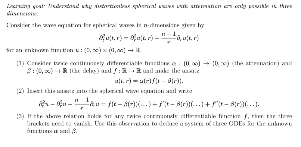
Consider the wave equation for spherical waves in $n$-dimensions given by
$$\partial_t^2u(t,r)=\partial^2_ru(t,r)+\frac{n-1}{r}\partial_ru(t,r)$$
for an unknown function $u:(0,\infty)\times(0,\infty)\rightarrow \mathbb{R}$

(1) Consider twice continuously differentiable functions $\alpha:(0,\infty)\rightarrow (0,\infty)$ (the attenuation) and $\beta:(0,\infty)\mathbb{R}$ (the delay) and $f:\mathbb{R}\rightarrow \mathbb{R}$ and make the ansatz
$$u(t,r)=\alpha(r)f(t-\beta(r))$$
(2) We insert this ansatz into the spherical wave equation
$$\partial_t^2\Big[\alpha(r)f(t-\beta(r))\Big]-\partial_r^2\Big[\alpha(r)f(t-\beta(r))\Big]-\frac{n-1}{r}\partial_r\Big[\alpha(r)f(t-\beta(r))\Big]$$
We compute the first term
$$\partial_t^2\Big[\alpha(r)f(t-\beta(r))\Big]\Rightarrow \boxed{\alpha(r)\partial_t^2f(t-\beta(r))}$$
The first derivative of the second term $$-\partial_r\Big[\alpha(r)f(t-\beta(r))\Big] =-\partial_r\alpha(r)f(t-\beta(r))+\alpha(r)\partial_r\beta(r)\partial_rf(t-\beta(r))$$
The derivative of the first term of the first derivative
$$-\partial_r^2\alpha(r)f(t-\beta(r))+\partial_r\alpha(r)\partial_r\beta(r)\partial_rf(t-\beta(r))$$
The derivative of the second term of the first derivative
$$\Big[\partial_r\alpha(r)\partial_r\beta(r)+\alpha(r)\partial^2_r\beta(r)\Big]\partial_rf(t-\beta(r))-\alpha(r)[\partial_r\beta(r)]^2\partial_r^2f(t-\beta(r))$$
That gives the second derivative of the second term $$\Rightarrow \boxed{-\partial_r^2\alpha(r)f(t-\beta(r))+\partial_r\alpha(r)\partial_r\beta(r)\partial_rf(t-\beta(r))}$$
$$\boxed{+\Big[\partial_r\alpha(r)\partial_r\beta(r)+\alpha(r)\partial^2_r\beta(r)\Big]\partial_rf(t-\beta(r))-\alpha(r)[\partial_r\beta(r)]^2\partial_r^2f(t-\beta(r))}$$
The third term:
$$-\frac{n-1}{r}\partial_r\Big[\alpha(r)f(t-\beta(r))\Big]\Rightarrow \boxed{-\frac{n-1}{r}\Big[\partial_r\alpha(r)f(t-\beta(r))-\alpha(r)\partial_r\beta(r)\partial_rf(t-\beta(r))\Big]}$$
We collect the coefficients of the $f(t-\beta(r))$ terms $$\partial_r^2\alpha(r)+\frac{n-1}{r}\partial_r\alpha(r)$$
and the coefficients of the $\partial_rf(t-\beta(r))$ terms
$$\partial_r\alpha(r)\partial_r\beta(r)\alpha(r)+\Big[\partial_r\alpha(r)\partial_r\beta(r)+\alpha(r)\partial^2_r\beta(r)\Big]+\frac{n-1}{r}\alpha(r)\partial_r\beta(r)$$
and the coefficients of the $\partial_r^2f(t-\beta(r))$ terms
$$\alpha(r)[\partial_r\beta(r)]^2-\alpha(r)$$
To make the brackets banish to zero, we set the three collections of terms equal to zero. Setting each collection of terms equal to zero gives the following system of ODEs
$$\boxed{\begin{cases}
\partial_r^2\alpha(r)+\frac{n-1}{r}\partial_r\alpha(r) =0 \\-2\partial_r\alpha(r)+\frac{n-1}{r}\alpha(r) =0\\
[\partial_r\beta(r)]^2=1
\end{cases}}$$
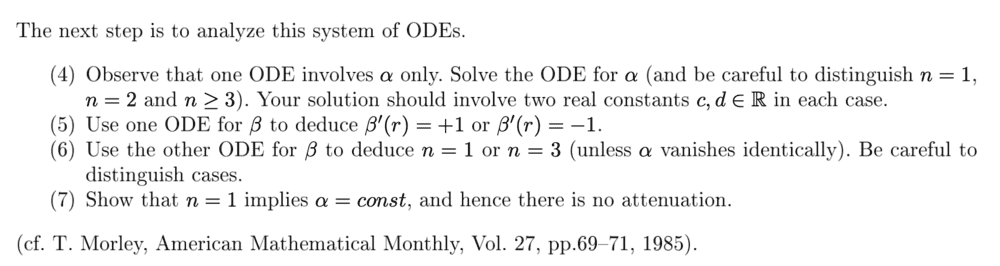
(4) The ODE that involves $α$only is $$\partial_r^2\alpha(r)+\frac{n-1}{r}\partial_r\alpha(r) =0$$
Case: $n=1$
$$\partial_r^2\alpha(r) =0$$
The roots of the characteristic polynomial $\lambda^2=0$ is just $0$. The solution is a polynomial of the form
$$\Rightarrow \boxed{\alpha(r)=cr+d} \quad \text{where }\quad c,d\in\mathbb{R}$$
setting $n=2$ gives a second order euler homegenuous ODE.
$$\partial_r^2\alpha(r)+\frac{1}{r}\partial_r\alpha(r) =0$$
The equation has a solution of the form $r^x$. plugging $r^x$ into the ODE gives the general solution
$$\boxed{\alpha(r)=cln(r)+d}$$
For the case $n\geq 3$ the ODE is
$$\partial_r^2\alpha(r)+\frac{2}{r}\partial_r\alpha(r) =0$$
By similar methods to the case $n=2$,
$$\boxed{\alpha(r)=\frac{c}{t}+d}$$
(5) The ODE for $β(r)$ is
$$[\partial_r\beta(r)]^2=1\Rightarrow \boxed{\partial_r\beta(r)=\pm 1}$$
(6) The following system of ODEs in $\alpha(r)$
$$\begin{cases}
\partial_r^2\alpha(r)+\frac{n-1}{r}\partial_r\alpha(r)=0\\
-2\partial_r\alpha(r)+\frac{n-1}{r}\alpha(r) =0\end{cases}$$ shows that there are no solutions, unless $n=1$ or $n=3$. We assume the solutions is of form $$\alpha(r)=cr^a$$ for some constants $c,a\in\mathbb{R}$.
Plugging in the solution to the system of ODEs gives
$$\begin{cases}
a(a-1)+(n-1)c=0 \\ -2a+(n-1)=0
\end{cases}$$
whose solution exists for $a$ only if $n=1$ or $n=3$.

(7) When we plug in $n=1$, we get $a=0$ which means $\alpha{r}=c$ for some $c\in\mathbb{R}$.edited: grammar

 

[haruspex]

The attenuation is the way the amplitude diminishes as the wave radiates out.
It is shown as a factor α(r), presumably monotonically decreasing.
The delay is the time lag between generation of a part of the wave and its reaching radius r. So again, it is a function of r, presumably monotonically increasing this time, with β(0)=0. It is subtracted from t in the expression for u(r,t).

If we have a bit of wave amplitude A emitted at time 0 (u(0,0)=A) and reaching radius r at time t = β(r) then its amplitude there and then will be u(r,t)=α(r)u(0, t-β(r))=α(r)u(0, 0)=Aα(r).