-02.2.11 initial value, graph, intervals xdx+ye^{-x}dy=0, \quad y(0)=1

[karush]

2000
(a) Find the solution of the given initial value problem in explicit form.
$$xdx+ye^{-x}dy=0, \quad y(0)=1$$
\begin{align*}\displaystyle
xdx&=-ye^{-x}dy \\
\frac{x}{e^{-x}}\, dx&=-y\, dy\\
xe^x\, dx&=-y\, dy
\end{align*}

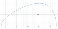
(b) Plot the graph of the solution
$\quad \textit{ok... I tried some attempts in W|A but my input didn't work}\\$
(c) Determine (at least approximately) the interval in which the solution is defined.
$\quad \textit{...provided by initial value!}$

View attachment 8664
​

 

[MarkFL]

(a) Find the solution of the given initial value problem in explicit form.
$$xdx+ye^{-x}dy=0, \quad y(0)=1$$
\begin{align*}\displaystyle
xdx&=-ye^{-x}dy \\
\frac{x}{e^{-x}}\, dx&=-y\, dy\\
xe^x\, dx&=-y\, dy
\end{align*}

(b) Plot the graph of the solution
$\quad \textit{ok... I tried some attempts in W|A but my input didn't work}\\$
(c) Determine (at least approximately) the interval in which the solution is defined.
$\quad \textit{...provided by initial value!}$

​

I would arrange the given ODE as:

\(\displaystyle y\,dy=-xe^x\,dx\)

Exchange dummy variables and integrate, using the given boundaries:

\(\displaystyle \int_1^y u\,dy=-\int_0^x ve^v\,dv\)

\(\displaystyle \frac{1}{2}(y^2-1)=-e^x(x-1)-1\)

\(\displaystyle y^2=-\left(2e^x(x-1)+1\right)\)

Given the initial value, we take the positive root:

\(\displaystyle y=\sqrt{-\left(2e^x(x-1)+1\right)}\)

Here's a plot:

View attachment 8665

The domain of the solution is found from:

\(\displaystyle -\left(2e^x(x-1)+1\right)\ge0\)

\(\displaystyle 2e^x(x-1)+1\le0\)

Using numeric techniques, we find (approximately):

\(\displaystyle -1.6783469900166606534\le x\le0.76803904701346556526\)

 

[karush]

total awsome

that was a great help let me see if I can do the next one...

which is.

$\quad\displaystyle
\frac{dr}{d\theta}=r^2/\theta
\quad r(1)=2$

Ill start a new thread tho
the $\theta$ scares me

 

[karush]

wait i don't think i see why the
intregration is set up the way it is,

never saw dummy variables

 

[MarkFL]

wait i don't think i see why the
intregration is set up the way it is,

never saw dummy variables

Suppose you have the initial value problem (IVP):

\(\displaystyle \frac{dy}{dx}=f(x)\) where \(\displaystyle y\left(x_0\right)=y_0\)

Now, separating variables and using indefinite integrals, we may write:

\(\displaystyle \int\,dy=\int f(x)\,dx\)

And upon integrating, we find

\(\displaystyle y(x)=F(x)+C\) where \(\displaystyle \frac{d}{dx}\left(F(x) \right)=f(x)\)

Using the initial condition, we get

\(\displaystyle y\left(x_0 \right)=F\left(x_0 \right)+C\)

Solving for \(C\) and using \(\displaystyle y\left(x_0\right)=y_0\), we obtain:

\(\displaystyle C=y_0-F\left(x_0 \right)\) thus:

\(\displaystyle y(x)=F(x)+y_0-F\left(x_0 \right)\)

which we may rewrite as:

\(\displaystyle y(x)-y_0=F(x)-F\left(x_0 \right)\)

Now, we may rewrite this, using the anti-derivative form of the fundamental theorem of calculus, as:

\(\displaystyle \int_{y_0}^{y(x)}\,dy=\int_{x_0}^{x}f(x)\,dx\)

Now, since the variable of integration gets integrated out, it is therefore considered a "dummy variable" and since it is considered good form not to use the same variable in the boundaries as we use for integration, we may switch these dummy variables and write:

\(\displaystyle \int_{y_0}^{y(x)}\,du=\int_{x_0}^{x}f(v)\,dv\)

This demonstrates that the two methods are equivalent.

Using the boundaries (the initial and final values) in the limits of integration eliminates the need to solve for the constant of integration, and I find it a more intuitive and cleaner approach to separable initial value problems.

 

[karush]

well that is pretty cool
most examples I saw had a lot of steps