Closed form not the same as the discrete form

[tworitdash]

clear;

lambda = 3e-2;

x = 4 * pi/lambda * linspace(eps, 15, 100000);

T = 5e-3;
t = [0:0.001e-3:T] ; % 0.1:1e-3:0.1+T];

u = 3;

a = 4*pi/lambda * u;

for i = 1:length(x)
    Z(i) = sum(-((cos(a.*t) - cos(x(i).*t)).^2 + (sin(a.*t) - sin(x(i).*t)).^2));
end

% Z1 = csc((a+x)/2) .* sin(1/2.*(2.*T + 1).*(a + x)) -1/2 .*  csc(a) .* sin(2.*a.*T+a) - 1/2 .* csc(x) .* sin(2.*T.*x+x)
Z1 = csc((a-x)/2) .* sin((T+1/2).*(a-x))/(2*pi) - 2*T - 1;

figure; plot(x*lambda/(4 * pi), (Z));
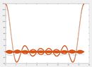
hold on; plot(x*lambda/(4 * pi), (Z1), '*');

<Moderator's note: CODE tags added. Please use them when posting code.>

The above code does two things. one is a summation over `t` and stores it in `Z` for all `x` individually with a for loop. The second thing it is doing is trying an analytical function for the summation in `t` and and just use the vector `x` to find the same quantity as `Z`, but analytically. it is stored in `Z1`. Somehow they both are not the same. The expression of the analytical form can be found in https://mathworld.wolfram.com/DeltaFunction.html equation (41) on that page. There is also a plot representing the function there. However, the MATLAB plot is very different. However, it is interesting to notice that `Z` and `Z1` are the same at the limiting case `a == x`. The plot I get is shown below. It should have a maximum at `a = x`, that is the value it should take at that point is `Z = Z1 = 0` and for the rest of the `x`, it should be less than 0. However, the blue plot satisfies it, but not the red one.

 

[DrClaude]

Z1 approaches a delta function as $T\rightarrow\infty$, you are using $T= 5 \times 10^{-3}$.