MATLAB IFFT doesn't match the analytical one

[tworitdash]

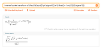
I have a Gaussian shape frequency domain spectrum of which I am calculating the Inverse Fourier transform. I use both IFFT of MATLAB and also an analytical expression of Mathematica. They are not the same.

I don't know where it is wrong. I have pasted both the figures. The numerical one has been zoomed in actually because the time domain pulse came out to be too thin. Any help is appreciated.The code is below:

clear;
% close all;lambda = 0.03;

PRT = 1e-3;
mu = 4; % Mean Doppler
sigma = 0.2;
v_amb = 7.5;

N = 60000; % Total number of points in time axis

t1 = 0:PRT:(N - 1)*PRT; % Time axis
vel_axis = linspace(-v_amb, v_amb, N); % velocity axis for the entire rotation

% vel_axis_hs = linspace(-v_amb, v_amb, hs); % velocity axis for one beamwidth
% t1 = -N/2*PRT:PRT:(N/2 - 1)*PRT; % Time axis
% s_analyt_o = 1./sqrt(2*pi*(sigma).^2) .* exp(-(vel_axis - mu).^2./(2*(sigma).^2));

% SNR = 10^(30/10);
% X = rand(1, N);
% Theta = 2 .* pi * rand(1, N);S_ = gaussmf(vel_axis, [sigma, mu]);

% Noise = sum(S_) ./ (N .* SNR);
% s_analyt_o = -(S_ + Noise) .* log(X);

s_analyt_o = S_;
s_num = ifft(ifftshift(sqrt(s_analyt_o))); % Numerical IFFTs_analyt = ifftshift((2/pi)^(1/4) * sqrt(sigma) .* exp(-t1 .* ((sigma)^2 .* t1 + 1j .* mu))); % analytical IFFT
figure; plot(t1, abs((s_analyt)));

figure; plot(t1, abs(ifftshift(s_num)));

 

[jasonRF]

This kind of problem depends on the details of what you are doing. If you provide a more clear description of exactly what you are trying to do, including equations and how you used Mathematica to compute the IFFT, it would be much easier to help. It is easy to have missing factors of $2 \pi$, $N$, etc, in amplitudes or function arguments. And I suspect that you used Mathematica to comput the inverse Fourier transform, not the inverse fast Fourier transform (IFFT) - yes?
Jason

 

[jedishrfu]

Also it would be nice if the diagrams were labeled so we know if they came from MATLAB or Mathematica.

 

[tworitdash]

This kind of problem depends on the details of what you are doing. If you provide a more clear description of exactly what you are trying to do, including equations and how you used Mathematica to compute the IFFT, it would be much easier to help. It is easy to have missing factors of $2 \pi$, $N$, etc, in amplitudes or function arguments. And I suspect that you used Mathematica to comput the inverse Fourier transform, not the inverse fast Fourier transform (IFFT) - yes?
Jason

I want to update some things in the question. I will make it clear, but I can't see the edit button anymore. Should I update the things in a new answer?

 

[Delta2]

I want to update some things in the question. I will make it clear, but I can't see the edit button anymore. Should I update the things in a new answer?

I think the edit option is lost in 24 hours after you initially post the message.
So
Either message a moderator (e.g. @Greg Bernhardt ) to restore the edit option (if that is possible, i am not sure)
Or just write a new post here.

 

[marcusl]

Shouldn’t you ifftshift after transforming, not before?

 

[tworitdash]

Now, I will write a more detailed explanation of what I was trying to do. I have considered a Gaussian-shaped spectrum for Doppler velocities that follows the following equation,

$$S(v) = \frac{1}{\sqrt(2\pi \sigma^2)} e^{-\frac{(v - \mu)^2}{2\sigma^2}}$$

Here,

It is assumed to be a group of scatters of different shapes and sizes moving with different velocities.

I want to see how does it look in the time domain when the radar is receiving this signal in slow time. As this is a power spectrum, for the time-domain we need the IDFT of the square root of this power spectrum (voltage equivalent).The pulse repetition time is 1 [ms], which corresponds to a pulse repetition frequency of 1 [kHz].

The velocity axis is,

$$v = [-\frac{\lambda}{4 \delta t}, \frac{\lambda}{4 \delta t})$$ with steps of $\frac{\lambda}{2 N \delta t}$.

The N is the number of pulses, the $\delta t$ is the pulse repetition time, $\lambda$ is the operating wavelength.

I approached it in two different ways. First, in MATLAB numerically using ifft function. Second, using MATLAB but analytical expression obtained from WolframAlpha (The mathematica engine). The screenshot is attached from Wolfram Alpha. As, in WolframAlpha it just converted from frequency to time, I used some modifications which may make it a velocity-time conversion.

The expression I used is this,

$$s(t) = (\frac{2}{\pi})^{1/4} \sqrt{\frac{2\sigma}{\lambda}} e^{-t ( (\sigma \frac{4\pi}{\lambda})^2 t + j \mu \frac{4\pi}{\lambda} )}$$The code is shown below.

clear;
% close all;lambda = 0.03;

PRT = 1e-3;
mu = 4; % Mean Doppler
sigma = 0.2;
v_amb = 7.5;

N = 60000; % Total number of points in time axis

t1 = 0:PRT:(N - 1)*PRT; % Time axis
vel_axis = linspace(-v_amb, v_amb, N); % velocity axis for the entire rotation

% vel_axis_hs = linspace(-v_amb, v_amb, hs); % velocity axis for one beamwidth
% t1 = -N/2*PRT:PRT:(N/2 - 1)*PRT; % Time axis
% s_analyt_o = 1./sqrt(2*pi*(sigma).^2) .* exp(-(vel_axis - mu).^2./(2*(sigma).^2));

% SNR = 10^(30/10);
% X = rand(1, N);
% Theta = 2 .* pi * rand(1, N);S_ = gaussmf(vel_axis, [sigma, mu]);

% Noise = sum(S_) ./ (N .* SNR);
% s_analyt_o = -(S_ + Noise) .* log(X);

s_analyt_o = S_;
s_num = ifft(ifftshift(sqrt(s_analyt_o))); % Numerical IFFTs_analyt = ((2/pi)^(1/4) * sqrt(sigma * 4 * pi / lambda) .* exp(-t1 .* ((sigma * 4 * pi / lambda)^2 .* t1 + 1j .* mu .* 4 * pi / lambda))); % analytical IFFT
figure; plot(t1, abs((s_analyt))/max(abs(s_analyt)), 'LineWidth', 2);

hold on; plot(t1, abs((s_num))/max(abs(s_num)), '*');
grid on;

xlim([-10 80]);

legend({'Wolfram Alpha Expression', 'MATLAB numerical'})

The results are shown. Here, I don't use any ifftshift. I have put one zoomed in image near time 0 and one at time 60 [sec]. These are the extreme time values. In the MATLAB one we see at both edges we have a pulse. However, we don't have it in the analytical one. It has the pulse only at 0.

 

[marcusl]

The Doppler shift from a moving target shows up in slow time as a phase shift from pulse to pulse, which you lose due to a conceptual issue--by starting with a power spectrum, you have no phase information at all. As a result, your estimate cannot reproduce the most important feature of the slow time data--the Doppler-induced phase shift.

 

[tworitdash]

The Doppler shift from a moving target shows up in slow time as a phase shift from pulse to pulse, which you lose due to a conceptual issue--by starting with a power spectrum, you have no phase information at all. As a result, your estimate cannot reproduce the most important feature of the slow time data--the Doppler-induced phase shift.

Good point. That I did only for the numerical one. Now, I multiplied a uniformly distributed random phase from $0$ to $2\pi$ with the square root of the power spectrum. I still get the same result because I am plotting the absolute values. To check if I have good phase information, I did the DFT again from these time-domain signals. I get the correct amplitude spectrum for both the analytical one and the numerical one.

My main problem is to find the time-domain equivalent of a Gaussian velocity spectrum. I proceed with this way but I am still not sure. That is why I checked for analytical solutions so that I can make a phase modulation later. I follow this paper to do the same. They start from a power spectrum. Then, they use a random phase that is uniformly distributed and multiply it with the square root of the power spectrum and then they do an IDFT to find the I and Q component of the time domain data.

https://journals.ametsoc.org/view/journals/apme/14/4/1520-0450_1975_014_0619_sowdsa_2_0_co_2.xml The code with the random phase in the amplitude spectrum is given below. It is a modified version.

clear;
% close all;lambda = 0.03;

PRT = 1e-3;
mu = 5; % Mean Doppler
sigma = 0.2;
v_amb = 7.5;

N = 60000; % Total number of points in time axis

t1 = 0:PRT:(N - 1)*PRT; % Time axis
vel_axis = linspace(-v_amb, v_amb, N); % velocity axis for the entire rotation

% vel_axis_hs = linspace(-v_amb, v_amb, hs); % velocity axis for one beamwidth
% t1 = -N/2*PRT:PRT:(N/2 - 1)*PRT; % Time axis
% s_analyt_o = 1./sqrt(2*pi*(sigma).^2) .* exp(-(vel_axis - mu).^2./(2*(sigma).^2));

% SNR = 10^(30/10);
% X = rand(1, N);
% Theta = 2 .* pi * rand(1, N);S_ = gaussmf(vel_axis, [sigma, mu]);

% Noise = sum(S_) ./ (N .* SNR);
% s_analyt_o = -(S_ + Noise) .* log(X);

s_analyt_o = S_;
s_num = ifft(ifftshift(sqrt(s_analyt_o) .* exp(1j .* 2 * pi * rand(1, N)))); % Numerical IFFTs_analyt = ((2/pi)^(1/4) * sqrt(sigma * 4 * pi / lambda) .* exp(-t1 .* ((sigma * 4 * pi / lambda)^2 .* t1 - 1j .* mu .* 4 * pi / lambda))); % analytical IFFT
figure;
plot(t1, abs((s_analyt))/max(abs(s_analyt)), 'LineWidth', 2);

hold on; plot(t1, abs((s_num))/max(abs(s_num)), '*');
grid on;

xlim([-10 80]);

legend({'Wolfram Alpha Expression', 'MATLAB numerical'})figure;

plot(vel_axis, abs(fftshift(fft(s_analyt)))/max(abs(fft(s_analyt)))); hold on;
plot(vel_axis, abs(fftshift(fft(s_num)))/max(abs(fft(s_num))));legend({'Wolfram Alpha Expression', 'MATLAB numerical'})

 

[marcusl]

Dusan Zrnic is a giant in the weather radar field (he literally wrote "the book" on Doppler weather radar), so you are looking at a good source.

 

[tworitdash]

Dusan Zrnic is a giant in the weather radar field (he literally wrote "the book" on Doppler weather radar), so you are looking at a good source.

Yes, it is a very good source indeed. My actual model is based on his idea from that paper. The problem I am facing is in the next step. This model of Zrnic is valid when the radar beam stays still and points to one direction in space. I am trying to create a model which considers the rotation of the beam with a beam width of roughly two degrees in azimuth. I can deduce the time domain signal for a monochromatic (Dirac) weather model in case of a rotating radar, but I am unable to do it for a Gaussian spectrum. I don't know how to modulate the time domain signal from this paper of Zrnic with a Gaussian Power spectrum to accommodate the rotation of the radar. Do you have any idea where can I find good sources for this kind of problem? This is the first step in my Ph.D. and I am unable to find a good reference for that. All references I found are more or less related to a rotating target with constant velocity, but no one talks about a distribution.