Conservation of probability issue when solving ODE in Mathematica

[kelly0303]

I am trying to solve this two level (Schrodinger) equation as a function of time:$$i\begin{pmatrix}
\dot{x}\\
\dot{y}
\end{pmatrix} = \begin{pmatrix}
0 & iW+dE_0sin(\omega t)\\
-iW+dE_0sin(\omega t) & \Delta
\end{pmatrix}\begin{pmatrix}
x\\
y
\end{pmatrix}$$

(I can go into more details about the Hamiltonian if needed). The initial conditions are $x(0)=1$, $y(0)=0$. This is my Mathematica code for it:

W = 10;
OmegaRabi = 1000;
omega = 700000;
delta = 10000;
eqns = {I*x'[t] == (I*W + OmegaRabi*Sin[omega*t])*y[t],
I*y'[t] == (-I*W + OmegaRabi*Sin[omega*t])*x[t] + y[t]*delta,
x[0] == 1, y[0] == 0};
sol = NDSolve[eqns, {x, y}, {t, 0, 4}][[1]]
Plot[{Abs[x[t]]^2 + Abs[y[t]]^2 /. sol}, {t, 0, 1}]

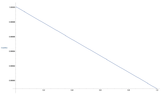
All the variables are as in the original equation except for OmegaRabi which is equal to $dE_0$. The output of this code (which would be the total probability i.e. $|x(t)|^2+|y(t)^2|$) should be constant 1. However I get what is seen in the plot below. I assume this has to do with some rounding numerical errors (?). Is there a way to fix it and ideally have it deviate from 1 much slower as a function of time? I am interested in the $|y(t)|^2$ as a function of time, and if one looks at that, the values for it are around 0.00002, so currently the error after one second seems to be 5 times bigger than the value I am interested in.

 

[DrClaude]

In NDSolve, you should modify AccuracyGoal and/or PrecisionGoal to try and get better results.