De Broglie–Bohm theory scattering from point charge, paths

[Spinnor]

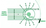
I think I read somewhere that the trajectories of particles in the De Broglie–Bohm theory do not cross, is that true?

If true, then in the case of Rutherford scattering the trajectories below can't be those of the De Broglie-Bohm theory?

Thanks.

 

[yucheng]

I believe the term "trajectory" in the two contexts, mean different things! Also, the "tranjectories" in the first image was calculated, but was the second picture also calculated, or is it just a high-school illustration? Hence you might not want to compare the two images. Pictures can be misleading!

P.S. would you state the source of the pictures?

 

[Spinnor]

I believe the term "trajectory" in the two contexts, mean different things! Also, the "tranjectories" in the first image was calculated, but was the second picture also calculated, or is it just a high-school illustration? Hence you might not want to compare the two images. Pictures can be misleading!

P.S. would you state the source of the pictures?

I believe the second image is an approximation of the classical calculation, it is exact in its approximation, it gets the main details correct.

Sources of images,

https://en.wikipedia.org/wiki/De_Broglie–Bohm_theory

https://www.geeksforgeeks.org/alpha-particle-scattering-and-rutherfords-nuclear-model-of-atom/

 

[Demystifier]

If true, then in the case of Rutherford scattering the trajectories below can't be those of the De Broglie-Bohm theory?

True. Even though classical and quantum physics predict the same differential cross section for scattering at the Coulomb potential, it's a coincidence without deeper meaning. The classical and quantum explanations of scattering are very different. If one takes the dBB picture merely as a thinking tool to visualize quantum physics in pseudo-classical terms (without any ontological commitment to the dBB interpretation claiming that Bohmian trajectories are "real"), one can use your example to visualize the difference between classical and quantum scattering.

 

[Demystifier]

Another example where the Bohmian trajectories are very different from classical trajectories is the Mach-Zehnder interferometer. If one attempts to reconstruct the particle trajectory from knowing which detector clicked, classical and Bohmian mechanics lead to the opposite conclusions.

 

[Spinnor]

If paths don't cross in the dBB interpretation, then in Rutherford scattering I think that must mean that those paths of closest impact parameter are deflected the least? Surely such a simple and important example must have been worked out? Thank you.

 

[Demystifier]

If paths don't cross in the dBB interpretation, then in Rutherford scattering I think that must mean that those paths of closest impact parameter are deflected the least?

Right.

Surely such a simple and important example must have been worked out? Thank you.

It should be straightforward, but I'm not aware that somebody has actually done it. If somebody wants to do that explicitly, it would be publishable. If somebody knows how to perform the computations but does not know hot to "sell it" as a paper worth publication, I can help as a coauthor.

 

[vanhees71]

The problem with Bohm's trajectories is that they are not observable. So why should one bother to do such a calculation?

 

[Demystifier]

The problem with Bohm's trajectories is that they are not observable. So why should one bother to do such a calculation?

1. In principle, Bohmian trajectories are observable by weak measurements.
2. Even without weak measurements (which would be difficult in this case) one can be motivated to do it for fun, to see how totally different trajectories (classical and Bohmian) can lead to the same differential cross section.

 

[vanhees71]

Measuring the trajectories of charged particles in Coulomb-scattering events would distort the cross section though!

 

[Demystifier]

Measuring the trajectories of charged particles in Coulomb-scattering events would distort the cross section though!

For ordinary "strong" measurements it's true. But for weak measurements it's not.

 

[gentzen]

Surely such a simple and important example must have been worked out?

It should be straightforward, but I'm not aware that somebody has actually done it. If somebody wants to do that explicitly, it would be publishable. If somebody knows how to perform the computations but does not know hot to "sell it" as a paper worth publication, I can help as a coauthor.

I guess that the De Broglie–Bohm trajectories actually do cross, and the challenge is less to compute trajectories doing something completely non-intuitive, but to explain why the image of the non-crossing trajectories behind the double slit is correct, despite the possibility for crossing in the general case.

Let me look at a simpler problem, the scattering of a particle on a potential barrier in 1D. Here it is totally obvious that the trajectories will cross whenever the particle is reflected. And here it is also totally obvious that the wavefunction of the incoming particle is not normalizable. So some window function must be used, ensuring that the wavefunction of the particle before the scattering is unambigously on one side (typically the left) of the potential barrier, and normalizable. This gives us a wavepacket that will scatter at the 1D barrier, and a distribution of Bohmian trajectories compatible with that wavepacket and its evolution. Some of those will be reflected and therefore cross itself, but the time dependence of the wavefunction resolves that paradox. And in the limit where the window function gets infinitely wide, regions where the trajectories don't cross emerge. The region behind the double slit is such a region.

 

[Demystifier]

Let me look at a simpler problem, the scattering of a particle on a potential barrier in 1D. Here it is totally obvious that the trajectories will cross whenever the particle is reflected.

In general, the claim that trajectories do not cross really means not cross at the same time. However, when the wave function is stationary, then they don't cross even at different times. In Coulomb scattering discussed above, a stationary wave function was implicitly assumed. In 1D, on the other hand, there is no scattering for stationary wave functions, so you implicitly assume a non-stationary one. In this case trajectories cross at different times, but not at the same time.

 

[Demystifier]

I guess that the De Broglie–Bohm actually do cross, and the challenge is less to compute trajectories doing something completely non-intuitive, but to explain why the image of the non-crossing trajectories behind the double slit is correct, despite the possibility for crossing in the general case.

For 1-particle case the Bohmian trajectories should be very intuitive, they are just integral curves of the probability current. In general, they never cross at the same time. In addition, when the wave function is stationary, they never cross even at different times.

 

[gentzen]

For 1-particle case the Bohmian trajectories should be very intuitive, they are just integral curves of the probability current. In general, they never cross at the same time. In addition, when the wave function is stationary, they never cross even at different times.

All the scenarios discussed here are stationary (stationary scattering problems), including the 1D scenario. But you have to interpret those scenarios as the limit of time dependent scenarios, in order to get a normalizable wavefunction.

The confusing part is that the trajectories themselves only depend on the phase of the wavefunction, and not on its absolute amplitude (not even locally). Behind the double slit, you are in the situation that the phases "converge" against a stable distribution in the limit, and therefore you get those non-crossing trajectories. But in the region where incoming and reflected wave overlap (in changing degrees) over time and interfere, it is at least not obvious whether such "simple" converence occurs too.

 

[Demystifier]

But in the region where incoming and reflected wave overlap over time and interfere, it is at least not obvious whether such "simple" converence occurs too.

Well, it's obvious to me. In one dimension the phase is some function $\varphi(x,t)$, so the velocity is $v(x,t)\propto\varphi'(x,t)$, where the prime denotes the derivative over $x$. Since $v(x,t)$ is a function, for any $(x,t)$ there is only one value of $v$. In other words, it's impossible to have two different $v$'s at the same $(x,t)$, i.e., at any $(x,t)$, two trajectories cannot cross.

 

[gentzen]

it is at least not obvious whether such "simple" converence occurs too.

Well, it's obvious to me.

I have the impression that you currently simply refuse to acknowledge the need of taking any limit at all. How can there be convergence, if no limit is involved at all? None of your formulas contain any parameter whose limit is investigated.

 

[Demystifier]

I have the impression that you currently simply refuse to acknowledge the need of taking any limit at all. How can there be convergence, if not limit is involved at all? None of your formulas contain any parameter whose limit is investigated.

Can you be more specific about your limit? I mean, can you express it with math, or with pictures, rather than with words?

 

[gentzen]

Can you be more specific about your limit? I mean, can you express it with math, or with pictures, rather than with words?

Take a "simple" window function, for example a (suitably shifted) Hann function ("raised cosine window"): $w_L(x):=\sin^2(\pi x/L) \chi_{(-L,0)}(x)$. Take $\phi_L(x,0):=w_L(x)\exp(ikx)$ to be the initial wavefunction, for the 1D scenario with a potential barrier starting at $x=0$. This initial wavefunction is now used both for the distribution of particles, and for solving the time dependent Schrödinger equation. For a given $L$, we get (a distribution of) trajectories, and those trajectories may cross each other, because of the time dependence. And now we investigate the limit for $L \to \infty$, especially the limit of the phase distribution of $\phi_L(x,t)$, where we are allowed to suppress a global phase factor like $\exp(-i\omega t)$.

 

[Demystifier]

Take a "simple" window function, for example a (suitably shifted) Hann function ("raised cosine window"): $w_L(x):=\sin^2(\pi x/L) \chi_{(-L,0)}(x)$. Take $\phi_L(x,0):=w_L(x)\exp(ikx)$ to be the initial wavefunction, for the 1D scenario with a potential barrier starting at $x=0$. This initial wavefunction is now used both for the distribution of particles, and for solving the time dependent Schrödinger equation. For a given $L$, we get (a distribution of) trajectories, and those trajectories may cross each other, because of the time dependence. And now we investigate the limit for $L \to \infty$, especially the limit of the phase distribution of $\phi_L(x,t)$, where we are allowed to suppress a global phase factor like $\exp(-i\omega t)$.

OK, let me present my educated guesses obtained intuitively, without actual computations. For large but finite $L$, the velocity function $v(x,t)$ changes slowly "everywhere", except close to the barrier where it changes fastly. So in the limit of infinite $L$, $v(x,t)$ is time-independent everywhere, except at $x=0$. Hence I expect something like
$$v(x,t)=u(x)+\delta(x) f(x,t)$$
where $u(x)$ and $f(x,t)$ are some well behaved functions. I repeat that those are educated guesses, which should be checked by actual calculations. Does it make sense?

 

[gentzen]

I repeat that those are educated guesses, which should be checked by actual calculations. Does it make sense?

The speed to the left of the potential barrier must be more complicated, because the reflected particles must be able to travel back.

I think what you actually get is that the time during which incident and reflected wavepacket overlap get longer and longer with $L\to \infty$.

 

[Demystifier]

I think what you actually get is that the time during which incident and reflected wavepacket overlap get longer and longer with $L\to \infty$.

Yes, that's probably true.