Is this algorithm stable? (time dependent diffusion equation)

[Telemachus]

Hi there. I was trying to solve the time dependent diffusion equation in only one dimension. I derived a explicit scheme using a finite difference in the time variable. The equation I am trying to solve is:

$\displaystyle \frac{1}{c} \frac{\partial \phi(x,t)}{\partial t} - \frac{\partial}{\partial x} \left( \kappa(x)\frac{\partial \phi(x,t)}{\partial x} \right) +\mu_a(x)\phi(x,t)=q(x,t)$.

I have used only an initial configuration to propagate: $\phi(x,t=0)=\phi(x)=-\frac{3}{200}x^4+15x$
I am also manufacturing analytic solutions, the solution I've proposed is: $\phi(x,t)=e^{-t}\left(-\frac{3}{200}x^4+15x\right)$

I use this solution to obtain the source on the right hand side of the diffusion equation, so then I have the analytic solution for that source. I've used inhomogeneus diffusion and absorption coefficients:

$\kappa(x)=\frac{x}{900}$
$\mu_a(x)=0.01\left(1+\frac{x}{10}\right)$

I've used an integral in the space variable such that: $f(x_j)=f_j=\frac{1}{\Delta x_j} \int_{x_{j-1/2}}^{x_{j+1/2}}f(x)dx$.

where $\Delta x_j=x_{j+1/2}-x_{j-1/2}=\Delta x\, \forall j$. This space discretization worked fine for the time independent equation, giving very good results even in very coarse grids.

According to a paper, with this spatial scheme and a forward, or backward finite difference in the time variable, the algorithm should be stable.

The explicit scheme looks at the end like this, for $x_j=(j-1)\Delta x$, $x_{j+1/2}=x_j+\frac{\Delta x}{2}$ and $t=(m-1)\Delta t$:

$\phi_j^{m+1} = \phi_j^{m} + c \Delta t \left[ q_j^m+\frac{1}{\Delta x^2} \left\{ \kappa_{j+1/2} ( \phi_{j+1}^m-\phi_j^m )-\kappa_{j-1/2} (\phi_j^m-\phi_{j-1}^m ) \right\}-\mu_{a,j} \phi_j^m \right]$

It wasn't really necessary, but as I was planning to work on implicit methods after this, I wrote the equation in matrix form, and solved it using matrix multiplication:

$\displaystyle \vec{\phi}^{m+1}=\left[\mathbb{\hat{1}}+c\Delta t \left( \hat A- \hat e_i \otimes \vec{\mu_a}\right) \right] \vec\phi^m+c\Delta t \vec{q}^m$.

I did a stability analysis using a discrete Fourier transform, but I couldn't get the dispersion relation, because I couldn't get the amplitudes separated in the equation, but the result I've got made me think that this scheme wasn't actually stable. When I wrote the code, and run it, it didn't seem to converge pretty well, I obtain some nonphysical negative scalar flux in the numeric solution:

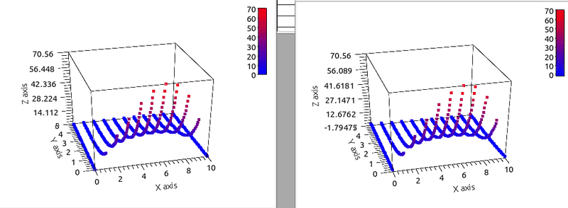
In the left is the analytic solution, and in the right the numerical. You can see that at the boundaries I have some negative values. I didn't use boundary conditions in the space variable, but I think I could do that, and fix the values at those points. The parameters I've used in this case are:

N= 10 M= 50 xmax=:10.000 dx= 1.0000 tmax=5.0000 dt= 0.10000 c= 10.000

N is the number of points in space, M the number of points in time. That solution looks fine, but if I use other values of c, it gets much worse. The solution blows up after some times steps. I thought of using more points, a finner grid, but instead of getting better, it gets actually worse, which really surprised me.

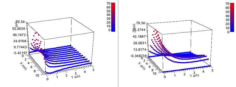
Here I plot for the same grid and c=1, and c=100:

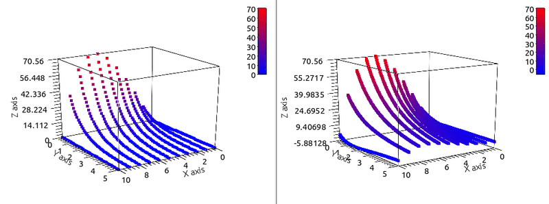
This last case is, in the left the analytical again, and in the right the numerical with:
N= 10 M= 400 xmax=:10.000 dx= 1.0000 tmax=5.0000 dt= 1.25000E-02c= 50.000

I didn't show it, but for other grids the solution explodes exponentially fast, I can't plot those cases.

When I tried to use the Von Neumann criteria for stability I got this expression for the dispersion relation:

$A(k)^2 = \displaystyle \left[ -\left(\kappa_{j+1/2}+\kappa_{j-1/2} \right) \cos(x)+ \kappa_{j+1/2}+\kappa_{j-1/2}-1+c\Delta t \frac{q(k)^m}{A(k)^m} - \mu_a(k) \right]^2+ \left(\kappa_{j+1/2}-\kappa_{j-1/2} \right)\sin^2(x)$.

The last term I think that can be dropped for smooth $\kappa$. But I'm not sure what conclusion to arrive with this last expression. It makes me think this isn't stable, on the one side because I don't think this is bounded to one. If there is stability, it must be conditioned stability and I don't know how to get the constraints from this expression. From the numerical experimentation there is clearly cases where this algorithm doesn't seem to be stable. The paper just mention the possibility of using a finite difference in time, but there are no citations, and actually uses other discretization, but pretty much complicated for the problem that it treats. I thought of starting with a explicit scheme because it is much simpler from an algebraic point of view.

I hoped to have some stability criteria that looked like some sort of Courant-Friedrichs-Lewy:

$\displaystyle \frac{c\kappa(x)\Delta t}{\Delta x} \leq 1$.

But I think that it is more complicated than that.

 

[Telemachus]

I had a silly mistake in the program. However, I still having some negatives values at x=0, but the program is much more stable. I have to ask a more mathematical question now, do I have to provide boundary conditions $\phi(x=0,t)$ and $\phi(x=10,t)\; \forall t$ or with the initial condition it should suffice $\phi(x,t=0)$?

 

[Telemachus]

Well, it worked after all. I had some other mistakes. I could propagate a vacuum with a delta source in space in time, and also relaxated a step function.

Here is the step function relaxed in time:

Due to the inhomogeneus diffusion and absorption it looks physically a reasonable solution.

Now I have written an implicit scheme which works better. This explicit scheme seems to have conditional stability, the usal Courant-Friedrichs-Lewy.