Tikz graph of y^3−3y^2−x−x^3+2=0, |x|<1

  • MHB
  • Thread starter karush
  • Start date
  • Tags
    Graph
In summary, plotting the equation $y^3-3y^2-x-x^3+2=0$ with the condition $|x|<1$ using TikZ is not possible. Instead, a parametrization can be used to plot the equation. One possible parametrization is $x = r(\phi)\cos\phi$ and $y = r(\phi)\sin\phi + 1$, where $r(\phi)=\sqrt{\frac{3\sin\phi+\cos\phi}{\sin^3\phi - \cos^3\phi}}$. Another parametrization that can be used is $x = (|q|-3)\cdot \tilde y(q)$ and
  • #1
karush
Gold Member
MHB
3,269
5
ok i tried to plot $y^3−3y^2−x−x^3+2=0, |x|<1$ but could not do so
spent about an hour trying to find a useable example but didn't

i am new to tikz but this is not a function...
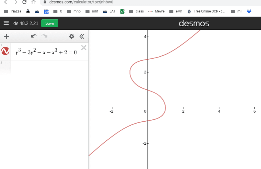
Screenshot 2020-07-16 at 1.55.48 PM.png


here is the code I tried. just borrowed a previos on i thot I could just replace the expression but no
\begin{tikzpicture}
%preamble \usepackage{pgfplots}
\begin{axis}[xmin=-1.8, xmax=1.8, ymin=-3, ymax=3, axis lines=middle, ticks=none]
\addplot[
draw=red, smooth, ultra thick, dashed,
domain=-1.5:1.5,
smooth
]{-x-x^3+2}
%{y^3−3y^2−x−x^3+2=0}
\foreach \x in {-1,0,1} { (axis cs:{\x},0) node[below right] {\x} };
\end{axis}
\end{tikzpicture}
 
Physics news on Phys.org
  • #2
TikZ does not support plotting graphs of equations natively.

Instead we can for instance parametrize the equation as:
\begin{cases}
x = r(\phi)\cos\phi \\
y = r(\phi)\sin\phi + 1
\end{cases}
where $r(\phi)=\sqrt{\frac{3\sin\phi+\cos\phi}{\sin^3\phi - \cos^3\phi}}$.

Then we can draw:
\begin{tikzpicture}[
declare function = {
radius(\phi)=sqrt((3*sin(\phi)+cos(\phi)) / (sin(\phi)^3 -cos(\phi)^3));
},
]
\draw[help lines] (-3,-2) grid (3,4);
\draw[->] (-3,0) -- (3.4,0);
\draw[->] (0,-2) -- (0,4.2);
\draw foreach \i in {-3,...,3} {(\i,-0.1) node[fill=black!5,below] {$\i$}};
\draw foreach \i in {-2,...,4} {(-0.1,\i) node[fill=black!5,left] {$\i$}};
\draw[domain=50:{atan(-1/3)+179.99}, variable=\phi, red, smooth, ultra thick] plot ({radius(\phi) * cos(\phi)}, {1 + radius(\phi) * sin(\phi)});
\draw[domain=-130:{atan(-1/3)-0.01}, variable=\phi, red, smooth, ultra thick] plot ({radius(\phi) * cos(\phi)}, {1 + radius(\phi) * sin(\phi)});
\end{tikzpicture}
 
Last edited:
  • #3
ok i was thinking doing that but wasn't sure how to set it up

i think many of the DE graphs will be like that

mahalo
 
  • #4
For reference, I derived the parametrization as follows.

We can see the point symmetry around (0,1) in the Desmos graph.
Shift the point of symmetry to the origin by introducing $\tilde y = y-1 \implies y = \tilde y + 1$.
Consequently we get:
\begin{aligned}y^3-3y^2-x-x^3+2&=
(\tilde y+1)^3-3(\tilde y+1)^2-x-x^3+2 \\
&=\tilde y^3+3\tilde y^2 +3\tilde y + 1 -3\tilde y^2 - 6\tilde y-3-x-x^3+2 \\
&=\tilde y^3-3\tilde y-x-x^3 \\
& = 0\end{aligned}

Substitute polar coordinates $x=r\cos\phi,\,\tilde y=r\sin\phi$ to get:
\[ \tilde y^3-3\tilde y-x-x^3=0 \\
(r\sin\phi)^3-3(r\sin\phi)-(r\cos\phi)-(r\cos\phi)^3=0 \\
r^3(\sin^3\phi - \cos^3\phi)=r(3\sin\phi+\cos\phi) \\
r=\pm \sqrt{\frac{3\sin\phi+\cos\phi}{\sin^3\phi - \cos^3\phi}} \quad\lor\quad r=0 \]

In polar coordinates we have that $r\ge 0$, so we will only have the $+$ solution.

Putting it together we get:
\begin{cases}x = r(\phi)\cos\phi \\ y=r(\phi)\sin\phi +1
\end{cases}
where $r(\phi)=\sqrt{\frac{3\sin\phi+\cos\phi}{\sin^3\phi - \cos^3\phi}}$.
 
Last edited:
  • #5
The question included the condition $|x|<1$, which we did not address yet.

I added that and improved the TikZ picture a bit:
\begin{tikzpicture}[
declare function = {
tilde_y(\q) = sign(\q)*sqrt(abs(\q) / (1 - (abs(\q)-3)^3));
},
pics/coordinates/.style args={(#1,#2),(#3,#4)}{ code={
\draw[help lines] (#1,#2) grid (#3,#4);
\draw[-latex] (#1,0) -- (#3,0);
\draw[-latex] (0,#2) -- (0,#4);
\node foreach \i in {#1,...,#3} at (\i,-0.1) [ below ] {$\i$};
\node foreach \i in {#2,...,#4} at (-0.1,\i) [ left ] {$\i$};
}},
every node/.style={fill=black!5},
fill=black!5,
]
\pic {coordinates={(-3,-2),(3,4)}};
\begin{scope}[draw=blue, ultra thick]
\draw[domain=-3.5:3.5, variable=\q, smooth] plot ({(abs(\q) - 3) * tilde_y(\q)}, {1 + tilde_y(\q)});
\filldraw foreach \p in {(1,3),(-1,2),(1,0),(-1,-1)} { \p circle (0.06) };
\end{scope}
\end{tikzpicture}

Just for fun, it uses a different parametrization that is based on slope.
We can find it by substituting $x=p\tilde y$ and solving for $\tilde y$ as function of $p$. It has $-3\le p<1$.
Afterwards I've reparametrized with $p=q-3$ to get a connected domain.

It is:
\begin{cases}x = (|q|-3)\cdot \tilde y(q) \\
y = \tilde y(q) + 1
\end{cases}
where $\tilde y(q)=\operatorname{sign}(q) \sqrt{\frac{|q|}{1-(|q|-3)^3}}$ and $-4<q<4$.
 
Last edited:
  • #6
Klaas van Aarsen said:
TikZ does not support plotting graphs of equations natively.

Instead we can for instance parametrize the equation as:
\begin{cases}
x = r(\phi)\cos\phi \\
y = r(\phi)\sin\phi + 1
\end{cases}
where $r(\phi)=\sqrt{\frac{3\sin\phi+\cos\phi}{\sin^3\phi - \cos^3\phi}}$.

Then we can draw:
\begin{tikzpicture}[
declare function = {
radius(\phi)=sqrt((3*sin(\phi)+cos(\phi)) / (sin(\phi)^3 -cos(\phi)^3));
},
]
\draw[help lines] (-3,-2) grid (3,4);
\draw[->] (-3,0) -- (3.4,0);
\draw[->] (0,-2) -- (0,4.2);
\draw foreach \i in {-3,...,3} {(\i,-0.1) node[fill=black!5,below] {$\i$}};
\draw foreach \i in {-2,...,4} {(-0.1,\i) node[fill=black!5,left] {$\i$}};
\draw[domain=50:{atan(-1/3)+179.99}, variable=\phi, red, smooth, ultra thick] plot ({radius(\phi) * cos(\phi)}, {1 + radius(\phi) * sin(\phi)});
\draw[domain=-130:{atan(-1/3)-0.01}, variable=\phi, red, smooth, ultra thick] plot ({radius(\phi) * cos(\phi)}, {1 + radius(\phi) * sin(\phi)});
\end{tikzpicture}
Klaas van Aarsen said:
The question included the condition $|x|<1$, which we did not address yet.

I added that and improved the TikZ picture a bit:
\begin{tikzpicture}[
declare function = {
tilde_y(\q) = sign(\q)*sqrt(abs(\q) / (1 - (abs(\q)-3)^3));
},
pics/coordinates/.style args={(#1,#2),(#3,#4)}{ code={
\draw[help lines] (#1,#2) grid (#3,#4);
\draw[-latex] (#1,0) -- (#3,0);
\draw[-latex] (0,#2) -- (0,#4);
\node foreach \i in {#1,...,#3} at (\i,-0.1) [ below ] {$\i$};
\node foreach \i in {#2,...,#4} at (-0.1,\i) [ left ] {$\i$};
}},
every node/.style={fill=black!5},
fill=black!5,
]
\pic {coordinates={(-3,-2),(3,4)}};
\begin{scope}[draw=blue, ultra thick]
\draw[domain=-3.5:3.5, variable=\q, smooth] plot ({(abs(\q) - 3) * tilde_y(\q)}, {1 + tilde_y(\q)});
\filldraw foreach \p in {(1,3),(-1,2),(1,0),(-1,-1)} { \p circle (0.06) };
\end{scope}
\end{tikzpicture}

Just for fun, it uses a different parametrization that is based on slope.
We can find it by substituting $x=p\tilde y$ and solving for $\tilde y$ as function of $p$. It has $-3\le p<1$.
Afterwards I've reparametrized with $p=q-3$ to get a connected domain.

It is:
\begin{cases}x = (|q|-3)\cdot \tilde y(q) \\
y = \tilde y(q) + 1
\end{cases}
where $\tilde y(q)=\operatorname{sign}(q) \sqrt{\frac{|q|}{1-(|q|-3)^3}}$ and $-4<q<4$.

wow yeah that adds a lot
there was a lot of code I haven't tried yet so mahalo
I did notice when it rendered in Overleaf that it was about twice the size needed by not sure if a scale down would be that easy
tying to avoid scaled images of graphs
usually don't put in grid just a few tics at critical points of intersection
also be nice to show both y and y' and their equations as labels

I am sure I can figure this out but would have not been able to do the parametric at my level
View attachment 10493
 
  • #7
karush said:
wow yeah that adds a lot
there was a lot of code I haven't tried yet so mahalo
I did notice when it rendered in Overleaf that it was about twice the size needed by not sure if a scale down would be that easy
tying to avoid scaled images of graphs
usually don't put in grid just a few tics at critical points of intersection
also be nice to show both y and y' and their equations as labels

I am sure I can figure this out but would have not been able to do the parametric at my level

I see where $|x|<1$ comes from now.
However, it is not enough to just restrict $x$. It also means that we have to restrict $y$ to the interval $(0,2)$.
That is because the top and bottom parts of the previous graph do not have $y(0)=1$, so they have to be left out.

Since $y'$ has a very different y-range, I guess it is best to put it in a separate graph.

Here's how we might do it with pgfplots:
\begin{tikzpicture}[
declare function = {
tilde_y(\q) = sign(\q)*sqrt(abs(\q) / (1 - (abs(\q) - 3)^3));
sol_x(\q) = (abs(\q)-3)*tilde_y(\q);
sol_y(\q) = tilde_y(\q) + 1;
derivative_y(\x,\y) = (1+3(\x)^2) / (3(\y)^2 - 6*(\y));
},
]
%preamble \usepackage{pgfplots}
\begin{axis}[
axis lines=middle,
ymax=2.4,
]
\addplot[red, domain=-2:2, smooth, ultra thick] ({sol_x(x)}, {sol_y(x)});
\addlegendentry{$y^3-3y^2=x^3+x-2$}
\end{axis}
\end{tikzpicture}
\begin{tikzpicture}[
declare function = {
tilde_y(\q) = sign(\q)*sqrt(abs(\q) / (1 - (abs(\q) - 3)^3));
sol_x(\q) = (abs(\q)-3)*tilde_y(\q);
sol_y(\q) = tilde_y(\q) + 1;
derivative_y(\x,\y) = (1+3(\x)^2) / (3(\y)^2 - 6*(\y));
},
]
%preamble \usepackage{pgfplots}
\begin{axis}[
axis lines=middle,
ymax=1.5,
]
\addplot[blue, domain=-2:2, smooth, ultra thick] ({sol_x(x)}, {derivative_y(sol_x(x), sol_y(x))});
\addlegendentry{$y'=\frac{1+3x^2}{3y^2-6y}$}
\end{axis}
\end{tikzpicture}
 
  • #8
Or alternatively we can do:
\begin{tikzpicture}[
declare function = {
tilde_y(\q) = sign(\q)*sqrt(abs(\q) / (1 - (abs(\q) - 3)^3));
sol_x(\q) = (abs(\q)-3)*tilde_y(\q);
sol_y(\q) = tilde_y(\q) + 1;
derivative_y(\x,\y) = (1+3(\x)^2) / (3(\y)^2 - 6*(\y));
},
]
\begin{scope}
\draw[-latex] (-1.5,0) -- (1.5,0);
\draw[-latex] (0,-8.5) -- (0,2.5);
\draw foreach \i in {-1} { (\i,0.1) -- (\i,-0.1) node[ below ] {$\i$} };
\draw foreach \i in {-8,-5,1,2} { (0.1,\i) -- (-0.1,\i) node[ left ] {$\i$} };
\begin{scope}[blue, thick]
\draw[domain=-2:2, variable=\q, smooth] plot ({sol_x(\q)}, {derivative_y(sol_x(\q),sol_y(\q))});
\draw[fill=black!5] foreach \p in {(-1,-8),(1,0)} { \p circle (0.06) } node[below right] {$y'$};
\end{scope}
\begin{scope}[red, thick]
\draw[domain=-2:2, variable=\q, smooth] plot ({sol_x(\q)}, {sol_y(\q)});
\draw[fill=black!5] foreach \p in {(-1,2),(1,0)} { \p circle (0.06) } node[above right] {$y$};
\end{scope}
\end{scope}
\end{tikzpicture}

It should scale just fine if you want to scale it.
 
  • #9
Klaas van Aarsen said:
Or alternatively we can do:
\begin{tikzpicture}[
declare function = {
tilde_y(\q) = sign(\q)*sqrt(abs(\q) / (1 - (abs(\q) - 3)^3));
sol_x(\q) = (abs(\q)-3)*tilde_y(\q);
sol_y(\q) = tilde_y(\q) + 1;
derivative_y(\x,\y) = (1+3(\x)^2) / (3(\y)^2 - 6*(\y));
},
]
\begin{scope}
\draw[-latex] (-1.5,0) -- (1.5,0);
\draw[-latex] (0,-8.5) -- (0,2.5);
\draw foreach \i in {-1} { (\i,0.1) -- (\i,-0.1) node[ below ] {$\i$} };
\draw foreach \i in {-8,-5,1,2} { (0.1,\i) -- (-0.1,\i) node[ left ] {$\i$} };
\begin{scope}[blue, thick]
\draw[domain=-2:2, variable=\q, smooth] plot ({sol_x(\q)}, {derivative_y(sol_x(\q),sol_y(\q))});
\draw[fill=black!5] foreach \p in {(-1,-8),(1,0)} { \p circle (0.06) } node[below right] {$y'$};
\end{scope}
\begin{scope}[red, thick]
\draw[domain=-2:2, variable=\q, smooth] plot ({sol_x(\q)}, {sol_y(\q)});
\draw[fill=black!5] foreach \p in {(-1,2),(1,0)} { \p circle (0.06) } node[above right] {$y$};
\end{scope}
\end{scope}
\end{tikzpicture}

It should scale just fine if you want to scale it.
yes I definitively like that one

mahalo for all the help,,, I'm going to continue more with these tikz graphs demos is really nice but there are features you want that it doesn't offer
 

1. What is a Tikz graph?

Tikz is a package in the LaTeX document preparation system that allows for the creation of high-quality, customizable graphs and diagrams.

2. How do I interpret the equation y^3−3y^2−x−x^3+2=0?

This equation represents a curve on a 2-dimensional coordinate plane, where the x-axis represents the values of x and the y-axis represents the values of y. The points on the curve satisfy the equation, meaning that when you plug in specific values for x and y, the equation will be true.

3. What does |x|<1 mean in this graph?

The vertical lines around the x in the equation represent the absolute value of x. This means that the graph only includes values of x that are less than 1 or greater than -1. In other words, the graph is limited to a specific range of x-values.

4. How do I plot this equation on a Tikz graph?

To plot this equation, you would use the Tikz package in a LaTeX document and input the equation into the appropriate command. You can also customize the graph by adjusting the scale, labels, and other features.

5. What does the graph of y^3−3y^2−x−x^3+2=0 look like?

Without seeing the specific graph, it is difficult to say exactly what it will look like. However, since this is a cubic equation, the graph will likely have a curved, "S" shape with multiple turning points. The graph will also be limited to a specific range of x-values due to the absolute value constraint.

Similar threads

  • MATLAB, Maple, Mathematica, LaTeX
Replies
4
Views
1K
  • MATLAB, Maple, Mathematica, LaTeX
Replies
1
Views
1K
  • MATLAB, Maple, Mathematica, LaTeX
Replies
5
Views
2K
  • MATLAB, Maple, Mathematica, LaTeX
Replies
7
Views
970
  • Poll
  • MATLAB, Maple, Mathematica, LaTeX
Replies
11
Views
2K
  • MATLAB, Maple, Mathematica, LaTeX
Replies
6
Views
1K
  • MATLAB, Maple, Mathematica, LaTeX
Replies
5
Views
2K
  • MATLAB, Maple, Mathematica, LaTeX
Replies
2
Views
741
  • MATLAB, Maple, Mathematica, LaTeX
Replies
2
Views
1K
  • MATLAB, Maple, Mathematica, LaTeX
Replies
1
Views
5K
Back
Top