What do "marginalized" or "marginalized error" mean? (contours - posterior)

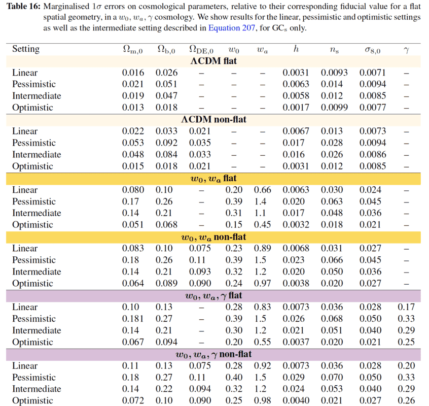
In summary: Evidence) and not a frequentist sense (marginalized... Probability) as I'm assuming.In summary, In summary, the table contains errors estimated on cosmological parameters with different confidence levels. The figure represents the correlations between the parameters. The figure also shows that the posterior distribution is obtained by inverting the Fisher's matrix. The other cases plotted in the figure represent joint distributions.
  • #1
fab13
312
6
TL;DR Summary
I would like to understand better the plotting of contours and the signification of the diagonal, .ie knowing if it corresponds to posterior distribution or not.
I am curently working on Forecast in cosmology and I didn't grasp very well different details.

Forecast allows, wiht Fisher's formalism, to compute constraints on cosmological parameters.

I have 2 issues of understanding :

1) Here below a table containing all errors estimated on these parameters, for different cases :
245904


In the caption of Table 16, I don't understand what the term "Marginalized 1##\sigma## erros" means. Why do they say "Marginalized", it could be simply formulated as "the constraints got with a ##1\sigma## confidence level" or ""errors with a ##1\sigma## C.L (68% of probability to be in the interval of values)", couldn't it ?If it would have been written "marginalized ##2\sigma## error, the first value in Table 16 would have been equal to ##(\Omega_{m,0})_{2\sigma}=0.032 = (\Omega_{m,0})_{1\sigma} =0.016 \text{x} 2##, wouldn't it be the case ?I would like to understand this vocabulary which is very specific of this Forecast field.2.1) Here below a figure representing the correlations (by drawing contours at ##1\sigma## and ##2\sigma## C.L (confidence levels)) between the different cosmological parameters :
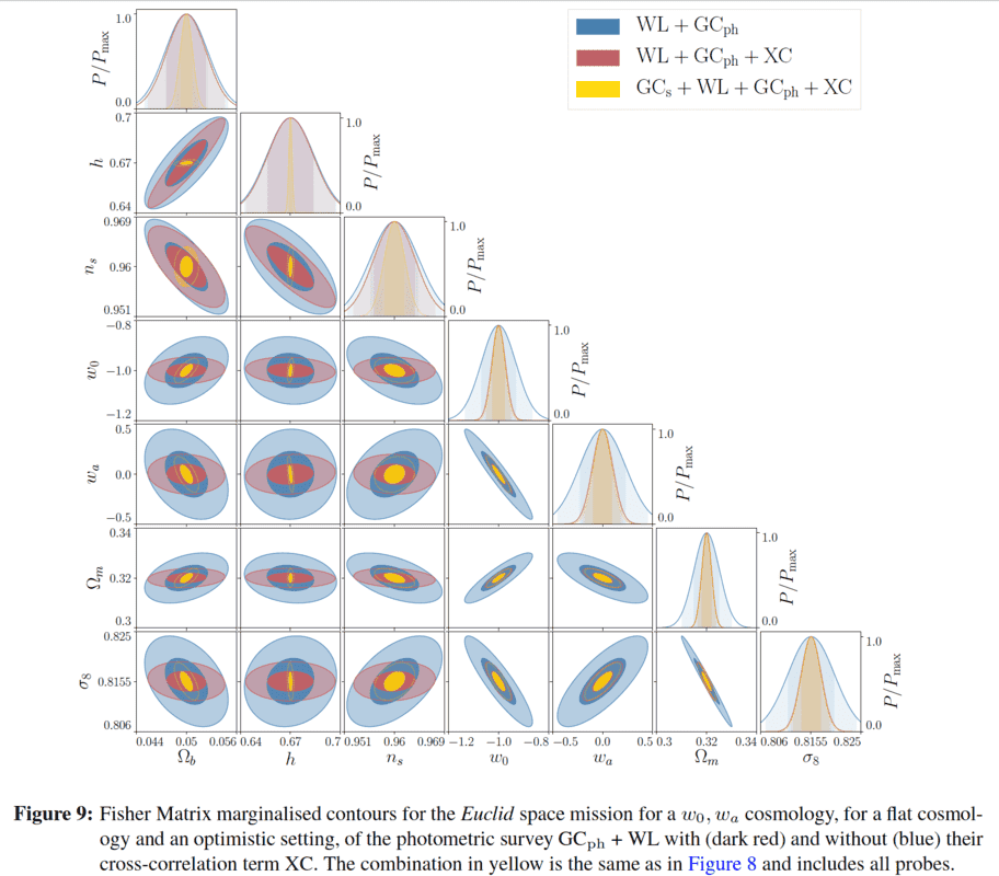
245905
I have understood, the right diagonal (with Gaussian shapes) represent the posterior distribution, i.e ##\text{Probability(parameters|data)}## or the probability to get an interval of values for each parameter, knowing the data.But how to justify that I have these posterior distribution on this descending diagonal ?I know the relation : ##\text{posterior}= \dfrac{\text{likelihood}\,\times\,\text{prior}}{\text{evidence}}## or the equivalent :##p(\theta|d)={\dfrac{p(d|\theta)p(\theta)}{p(d)}}## with ##\theta## the parameters and ##d##the data.We can use Fisher's formalism assuming likelihood is Gaussian, and the posterior are obtained by inverting the Fisher's matrix.So I wonder what are the others cases (except this diagonal) plotted and mosty what they represent in the formula above, especially towards posterior distribution :##\text{posterior}= \dfrac{\text{likelihood}\,\times\,\text{prior}}{\text{evidence}}##It seems all this cases looks like "joint distribution" but I can't get to recall what this joint distribution corresponds to, and its link with posterior distribution.2.2) Finally, a last question, in the caption of figure 9, it is also noted "marginalized contours" : there too, why using the term "marginalized" ??Any help is welcome, I would be very grateful.If someone thinks this post should be moved to another forum, don't hesitate to do it. I posted here since there is a physical context but I may be wrong.Regardsps : GC represents Galaxy clustering probe, WL the weak lensing, GC##_{\text{ph}}## the photometric proble and XC the cross-correlations.
 
Space news on Phys.org
  • #2
1. Marginalised means that you have integrated out all other parameters. In other words, it is the distribution of a single (or two in the case of a two dimensional marginalised distribution) parameter after integrating over the others. This is in stark contrast to frequentist statistics, where marginalisation does not make sense in the same fashion and you would instead do profiling.

Also note that Bayesian statistics does not have confidence levels - that is a frequentist concept. Instead, Bayesian statistics consider credible regions (or intervals in one dimension).

2.1. Again note the issue of confidence (frequentist) versus credibility (Bayesian).

You cannot have the posterior without having the actual data. However, you can predict the posterior under some assumptions. Those assumptions should be stated in the reference.

Regarding the figure, you can make such plots for any distribution. It shows you the marginalised distribution. On the diagonal you find the distribution marginalised to a single parameter and on the off-diagonal marginalised to two parameters (all other parameters have been integrated over the distribution).

2.2) Again, marginalising means integrating out parameters not shown over the corresponding distribution.
 
  • #3
@Orodruin thanks for your quick answer.

1) Concerning the descending diagonal on the right , does it represent a distribution in a frequentist sense or bayesian sense ?

We agree this diagonal represent the posterior of each parameter, i.e the probability (by integrating the surface of PDF) to have the parameter into a range (i.e, bounds of integration) knowing the data, don't we ? In my case, the data come from CAMB code which produces matter power spectrum.

2) So, assuming the fact that posteriors are represented on this diagonal, I don't understand how to introduce the notion of integration over all others parameters ?

Could you take a concrete example of integration on a posterior distribution ? (I make confusions between PDF of a random variable and the posterior of this random variable)

3) When we talk about frequentist way, I understand that marginalization is done by : ##f(x)=\int_{0}^{+\infty}f(x,y)\,\text{d}y## but I can't get to do the same wih posterior ##p(\theta|d)## (with ##p(\theta|d)=\dfrac{p(d|\theta)p(\theta)}{p(d)}## ).

Indeed, in frequentist way, we manipulate PDF when we perform integration whereas in Bayesian approach, we manipulate probability and I don't know how to handle the marginalisation of a paramater whose I only know the probability and not its PDF.

That's why I would like to give me a simple and concrete example of marginalization (in Bayesian approach) by integrating over all others parameters with the definition of posterior probability that I have written above ?

4) Unless, diagonal cases has only a Bayesian sense (posterior distribution) whereas all off-diagonal cases have a frequentist sense (i.e the representation of 2 PDF in 2D plane of parameters) ?

Sorry if the answers about these questions are evident but this is a new field for me.

Regards
 
Last edited:
  • #4
1) There is only the Bayesian sense. In the frequentist approach there is no parameter distribution. The diagonal shows the marginalised 1D distribution. I am just saying ”distribution” because in general you can do plots like this for any distribution, whether prior or posterior.

2) What is shown in the figure are the marginalised distributions. In other words, the other parameters have already been integrated out.

3) You do not do marginalisation of parameters in the frequentist picture because you do not have probability distributions for the parameters. You can do marginalisation for any PDF, the posterior is a PDF.

4) No, you are not mixing Bayesian and frequentist. Everything is Bayesian. The off-diagonals show credible regions of the 2D marginalised distributions.
 
  • #5
@Orodruin : ok, thanks for your patience

1) Sorry, I didn't know that, in frequentist field, the notion of PDF (probability density function) doesn't exist.

What are the parameters which are used currently in frequentist domain : expectation, standard deviation ... ? Could you give me fundamentals and importrant parameters in this field ?

2) When you say that marginalised distribution corresponds when all other parameters have been already integrated out : for example, in the case of 2 parameters (off-diagonal cases in my figure), If I know the joint 2D probalbility ##g(x,y)## of the 2 random variables ##X## and ##Y##, can I write the marginal distribution on parameter ##X## like this ;

##f(x)=\int_{0}^{+\infty}g(x,y)\,\text{d}y##

By the way, does one say "marginal distribtion on ##X## or "marginal distribtion on ##Y## parameter ? I mean, have I to precise the parameter that I ntegrate (##Y## ?) or the paramater which is described by the PDF ##f(x)##

3) Into my case, the operation of integration that we talk about is done on the posterior (it's a PDF) :

So to marginalise , if I understand well, I compute the likelihood ##p((X,Y)|d)## and after, I integrate on ##Y## random variable ? like this ;

##p(X|d)=\dfrac{p(d|X)p(X)}{p(d)}= \int_{0}^{+\infty}\,p((X,Y)|d) \text{d}y## ? is it right ?

If this is wrong, could you give please an example of quantity that I have to integrate (posterior distribution, likelihood ...?) to get a marginalised distribution on only 1 parameter (all others have disappeared since the integration)

4) You say, that in Bayesian school of thoughts, Confidence level doesn't exist : Indeed in frequentist domain, we have the formula :

##I_{c}=\left[{\bar{x}}-t_{\alpha}{\frac{s}{\sqrt{n}}}\ ;\ {\bar{x}}+t_{\alpha}{\frac{s}{\sqrt{n}}}\right]##

which gives the interval of confidence level : What's the link between C.L interval and Credibility interval (that we find in Bayesian approach). It would be interesting to grasp these differences.

For example, the definition of a confidence levl C.L with ##\chi^2## is given by :

##1-CL={\large\int}_{\Delta\chi^{2}_{CL}}^{+\infty}\,\dfrac{1}{2}\,e^{-\dfrac{\Delta\chi^{2}}{2}}\,d\,\chi^{2}=e^{-\dfrac{\Delta\chi_{CL}^{2}}{2}}##

So this definition sould be a frequentist approach, shouldn't it ? However, I have taken in this formula the PDF of the ##\chi^{2}##.

Regards
 
  • #6
fab13 said:
Sorry, I didn't know that, in frequentist field, the notion of PDF (probability density function) doesn't exist.
It does, but not for parameters. When dealing with parameter estimation in the frequentist setting, you use confidence intervals and confidence levels - not probability distributions for the parameters.

2) You would say "the probability distribution of x, marginalised over y" if you want to be clear.

3) Yes.

fab13 said:
What's the link between C.L interval and Credibility interval (that we find in Bayesian approach). It would be interesting to grasp these differences.
There is no link, that is the point. They have similar usage in the different approaches and in some idealised cases they will turn out to be the same. However, the interpretation is fundamentally different due to the fundamental differences between frequentist and Bayesian statistics.
 
  • #7
do you agree with the formula in 3) ? , i.e :

##p(X|d)=\dfrac{p(d|X)p(X)}{p(d)}= {\large\int}_{0}^{+\infty}\,p((X,Y)|d) \text{d}y={\large\int}_{0}^{+\infty}\dfrac{p(d|(X,Y))p((X,Y))}{p(d)} \text{d}y##

1) Indeed, I am looking for where the integration is performed when we want to marginalise

2) When you talk about parameter, you want to talk about a random variable : this is the same thing ?

Regards
 
  • #8
No, I do not agree with the second line, because you cannot predict the data from x alone. Therefore there is no such thing as p(d|X). The rest is fine.

1) The integration is the marginalisation.

2) No it is not. A parameter is a model parameter that given your model can be used to predict the distribution of the data. In Bayesian statistics, model parameters have a probability distribution. In frequentist statistics they do not.
 
  • #9
in the following formula :

##p(X|d)=\dfrac{p(d|X)p(X)}{p(d)}= {\large\int}_{0}^{+\infty}\,p((X,Y)|d) \text{d}y={\large\int}_{0}^{+\infty}\dfrac{p(d|(X,Y))p((X,Y))}{p(d)} \text{d}y##

The factor ##p(d|X)## is commonly taken as the likelihood function : this assumes a theoritical model on ##X## from which we can produce data with the theoritical likelihood and that's why I write ##p(d|X)##=probability of having data given a model for the distribution of X (which is a parameter in Bayesian approach and not a random variable like in Frequentist approach, is it good ??).

Do you understand better why I want to know exactly at which step the marginalisation/integration is performed.

your explanations are precious since I am taking over my studies in a master degree and I am so an old student :), thanks
 
Last edited:
  • #10
fab13 said:
in the following formula :

##p(X|d)=\dfrac{p(d|X)p(X)}{p(d)}= {\large\int}_{0}^{+\infty}\,p((X,Y)|d) \text{d}y={\large\int}_{0}^{+\infty}\dfrac{p(d|(X,Y))p((X,Y))}{p(d)} \text{d}y##

The factor ##p(d|X)## is commonly taken as the likelihood function : this assumes a theoritical model on ##X## from which we can produce data with the theoritical likelihood and that's why I write ##p(d|X)##=probability of having data given a model for the distribution of X (which is a parameter in Bayesian approach and not a random variable like in Frequentist approach, is it good ??).

Do you understand better why I want to know exactly at which step the marginalisation/integration is performed.

your explanations are precious since I am taking over my studies in a master degree and I am so an old student :), thanks

1) I have changed the notations since there could be confusions between a random variable ##X## or ##Y## and a parameter. So, I replaced ##X## by ##\theta_{1}## and ##Y## by parameter ##\theta_{2}##; this way, I can reformulate above like this :

##p(\theta_{1}|d)=\dfrac{p(d|\theta_{1})p(\theta_{1})}{p(d)}= {\large\int}_{0}^{+\infty}\,p((\theta_{1},\theta_{2})|d) \text{d}\theta_{2}={\large\int}_{0}^{+\infty}\dfrac{p(d|(\theta_{1},\theta_{2}))p((\theta_{1},\theta_{2}))}{p(d)} \text{d}\theta_{2}##

The factor ##p(d|\theta_{1})## is commonly taken as the likelihood function : this assumes a theoritical model on ##\theta_{1}## from which we can produce data with the theoritical likelihood and that's why I write ##p(d|\theta_{1})##=probability of having data given a model for the distribution of \theta_{1} (which is a parameter in Bayesian approach and not a random variable like in Frequentist approach, is it good ??).

2) In order to express explicity the marginalisation, I don't know if I have made an error in the following relation cited above, i.e ##(1)## :

##p(\theta_{1}|d)=\dfrac{p(d|\theta_{1})p(\theta_{1})}{p(d)}= {\large\int}_{0}^{+\infty}\,p((\theta_{1},\theta_{2})|d) \text{d}\theta_{2}={\large\int}_{0}^{+\infty}\dfrac{p(d|(\theta_{1},\theta_{2}))p((\theta_{1},\theta_{2}))}{p(d)} \text{d}\theta_{2}\quad(1)##

Indeed, shouldn't we have to write instead of it the following relation ? :

##p(d|\theta_{1})= {\large\int}_{0}^{+\infty}\,p(d|(\theta_{1},\theta_{2})) \text{d}\theta_{2}={\large\int}_{0}^{+\infty}\dfrac{p((\theta_{1},\theta_{2})|d))\,p(d)}{p((\theta_{1},\theta_{2})}##

and finally get :

##p(d|\theta_{1})= {\large\int}_{0}^{+\infty}\,\dfrac{p((\theta_{1},\theta_{2})|d)\,p(d)}{p((\theta_{1},\theta_{2})} \text{d}\theta_{2}##

which implies :

##p(\theta_{1}|d)= \bigg[{\large\int}_{0}^{+\infty}\,\dfrac{p((\theta_{1},\theta_{2})|d)\,p(d)}{p((\theta_{1},\theta_{2})} \text{d}\theta_{2}\bigg]\,\dfrac{p(\theta_{1})}{p(d)}\quad(2)##Are both equations (1) and (2) relations correct ?

3) In practise, if both (1) and (2) are correct, I would prefer to use equation(1) since I can compute ##p(d|(\theta_{1},\theta_{2}))## from the likelihood with a theoritical model for parameters ##\theta_{1}## and ##\theta_{2}##, and also with uniform prior for ##p(\theta_{1},\theta_{2})## :

what do you think about ?
 
Last edited:
  • #11
Sorry, there is a missing ##\text{d}\theta_{2}## in the equation :

##p(d|\theta_{1})= {\large\int}_{0}^{+\infty}\,p(d|(\theta_{1},\theta_{2})) \text{d}\theta_{2}={\large\int}_{0}^{+\infty}\dfrac{p((\theta_{1},\theta_{2})|d))\,p(d)}{p((\theta_{1},\theta_{2})}\,\text{d}\theta_{2}##
 
  • #12
I don't want to be too insistent but could anyone confirm to me the validity of the following relations above ##(1)## and ##(2)## :

##p(\theta_{1}|d)=\dfrac{p(d|\theta_{1})p(\theta_{1})}{p(d)}= {\large\int}_{0}^{+\infty}\,p((\theta_{1},\theta_{2})|d) \text{d}\theta_{2}={\large\int}_{0}^{+\infty}\dfrac{p(d|(\theta_{1},\theta_{2}))p((\theta_{1},\theta_{2}))}{p(d)} \text{d}\theta_{2}\quad(1)##

and

##p(\theta_{1}|d)= \bigg[{\large\int}_{0}^{+\infty}\,\dfrac{p((\theta_{1},\theta_{2})|d)\,p(d)}{p((\theta_{1},\theta_{2})} \text{d}\theta_{2}\bigg]\,\dfrac{p(\theta_{1})}{p(d)}\quad(2)##

assuming, in practise, that I know the theoretical model which allows me to compute ##\text{Probability(data|parameter)}##, i.e I could get this by computing the likelihood for this probability.

But last point, relations ##(1)## and ##(2)## seems to be difficult to compute since I don't think I can take a uniform distribution for the factor ##p(\theta_{1},\theta_{2})## : is it really the case ?

Thanks for your help.
 

What does "marginalized" mean in the context of scientific research?

In scientific research, the term "marginalized" refers to the exclusion or neglect of a particular group or factor in the analysis or interpretation of data. This can lead to biased or incomplete conclusions.

What is a "marginalized error" in scientific studies?

A "marginalized error" is an error or bias that occurs when a particular group or factor is not adequately considered in the research process. This can lead to incorrect or misleading conclusions.

How do researchers account for marginalized factors in their studies?

Researchers can account for marginalized factors by actively seeking out diverse perspectives and including them in the research design, data collection, and analysis. This can help to minimize bias and provide a more comprehensive understanding of the topic.

What role do "contours" play in understanding marginalized groups in scientific research?

In scientific research, "contours" refer to the boundaries or limits of a particular phenomenon or group. By examining the contours of marginalized groups, researchers can gain a better understanding of their experiences and perspectives, which can inform more inclusive and accurate research.

How does considering marginalized factors contribute to the overall scientific knowledge?

Considering marginalized factors in scientific research can contribute to a more comprehensive and accurate understanding of a topic. It can also help to identify and address systemic inequalities and promote more inclusive and ethical research practices.

Similar threads

Replies
5
Views
917
  • Set Theory, Logic, Probability, Statistics
Replies
1
Views
964
  • Set Theory, Logic, Probability, Statistics
Replies
6
Views
738
Replies
1
Views
1K
  • Set Theory, Logic, Probability, Statistics
Replies
16
Views
1K
  • Set Theory, Logic, Probability, Statistics
Replies
1
Views
769
  • Set Theory, Logic, Probability, Statistics
Replies
11
Views
1K
  • Set Theory, Logic, Probability, Statistics
Replies
1
Views
1K
  • Advanced Physics Homework Help
Replies
2
Views
2K
Back
Top