1D Convection Diffusion Equation - Inlet Mixing Effect

Click For Summary
SUMMARY

The forum discussion centers on solving the 1D convection-diffusion equation using a Matlab code with the Crank-Nicolson scheme, specifically for modeling a sensible stratified storage tank. The user encounters an abnormal temperature increase when incorporating an effective diffusivity factor (εeff) with a hyperbolic decaying form. Despite attempts with various finite difference methods, including Forward-Time Central Space and Crank-Nicolson with Upwind Treatment, the issue persists. The discussion highlights the need for a more accurate formulation of the diffusion term to mitigate numerical dispersion and improve solution accuracy.

PREREQUISITES
  • Matlab programming for numerical simulations
  • Understanding of the Crank-Nicolson scheme for solving PDEs
  • Knowledge of finite difference methods in numerical analysis
  • Familiarity with convection-diffusion equations and thermal diffusivity concepts
NEXT STEPS
  • Review the formulation of the diffusion term in convection-diffusion equations
  • Learn about numerical dispersion and its impact on finite difference methods
  • Explore advanced numerical techniques for solving PDEs, such as the method of characteristics
  • Investigate the implementation of spatially varying diffusivity in numerical simulations
USEFUL FOR

Researchers, engineers, and students working on fluid dynamics, thermal analysis, or numerical methods in engineering, particularly those involved in modeling convection-diffusion processes.

HumanistEngineer
Messages
18
Reaction score
2
I have a working Matlab code solving the 1D convection-diffusion equation to model sensible stratified storage tank by use of Crank-Nicolson scheme (without εeff in the below equation).

2018-07-24_14_43_59-_Zurigat_et_al_AE_1988.pdf.png


As indicated by Zurigat et al; there is an additional mixing effect having a hyperbolic decaying form from the top of the tank to the bottom (at the inlet we have a high rate of mixing). So I try to involve εeff as a magnifying effect on the thermal diffusivity as shown in the equation above. Please see the section Inlet Mixing in the Matlab code below.

The problem is that: there occurs an abnormal temperature increase more than the coming inlet temperature whenever I involve the mixing effect as a hyperbolic decaying form (please see pictures below).

Would you please tell me why I have this abnormal temperature increase problem? I tried also Forward-Time Central Space method and CN with upwind treatment but at all approaches, I encountered this abnormal issue. Any solution please? I am not so experienced with the finite difference methods!

With εeff involved, the problem with abnormal temperature increase encountered:
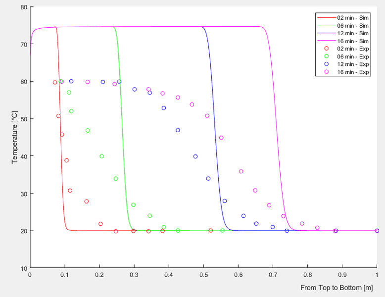
2018-07-24_14_58_12-_Figures_-_Figure_1.png


The case without εeff, the solution of convection-diffusion equation for a stratified sensible storage tank by use of Crank-Nicolson scheme:
2018-07-24_14_19_45-_Figures_-_Figure_1.png


Matlab Code:

Code:
function [T,dh,dt] = CDR_CrankNicolson_Exp_InletMixing(t_final,n)
%% 1D Convection-Diffusion-Reaction (CDR) equation - Crank-Nicolson scheme
%   solves a d2u/dx2 + b du/dx + c u = du/dt

%% References
% pg. 28 - http://www.ehu.eus/aitor/irakas/fin/apuntes/pde.pdf
% pg. 03 - https://www.sfu.ca/~rjones/bus864/notes/notes2.pdf
% http://nptel.ac.in/courses/111107063/24

tStart = tic; % Measuring computational time

%% INPUT
% t_final   : overall simulation time [s]
% n         : Node number [-]

%% Tank Dimensions
h_tank=1;       % [m]       Tank height
d_tank=0.58;     % [m]       Tank diameter
vFR=11.75;        % [l/min]   Volumetric Flow Rate
v=((vFR*0.001)/60)/((pi*d_tank^2)/4);    % [m/s]     Water velocity

dh=h_tank/n;       % [m] mesh size

dt=1;             % [s] time step
maxk=round(t_final/dt,0);    % Number of time steps

% Constant CDR coefficients | a d2u/dx2 + b du/dx + c u = du/dt
a_const=0.15e-6;     % [m2/s]Thermal diffusivity
b=-v;                        % Water velocity
c=0;                         %! Coefficient for heat loss calculation

%% Inlet Mixing - Decreasing hyperbolic function through tank height
eps_in=2;             % Inlet mixing magnification on diffusion
A_hyp=(eps_in-1)/(1-1/n);
B_hyp=eps_in-A_hyp;

Nsl=1:1:n;

eps_eff=A_hyp./Nsl+B_hyp;

a=a_const.*eps_eff;         % Case 0
% a=ones(n,1)*a_const;      % Case 1
% a=ones(n,1)*a_const*20;    % Case 2

%% Initial condition - Tank water at 20 degC
T=zeros(n,maxk);

T(:,1)=20;

%% Boundary Condition - Inlet temperature at 60 degC
T(1,:)=60;

%% Formation of Tridiagonal Matrices
%   Tridiagonal Matrix @Left-hand side
subL(1:n-1)=-(2*dt*a(1:n-1)-dt*dh*b);             % Sub diagonal - Coefficient of u_i-1,n+1
maiL(1:n-0)=4*dh^2+4*dt*a-2*dh^2*dt*c;          % Main diagonal - Coefficient of u_i,n+1
supL(1:n-1)=-(2*dt*a(1:n-1)+dt*dh*b);             % Super diagonal - Coefficient of u_i+1,n+1
tdmL=diag(maiL,0)+diag(subL,-1)+diag(supL,1);
%   Tridiagonal Matrix @Right-hand side
subR(1:n-1)=2*dt*a(1:n-1)-dt*dh*b;                % Sub diagonal - Coefficient of u_i-1,n
maiR(1:n-0)=4*dh^2-4*dt*a-2*dh^2*dt*c;          % Main diagonal - Coefficient of u_i,n
supR(1:n-1)=2*dt*a(1:n-1)+dt*dh*b;               % Super diagonal - Coefficient of u_i+1,n
tdmR=diag(maiR,0)+diag(subR,-1)+diag(supR,1);

%% Boundary Condition - Matrices
tdmL(1,1)=1; tdmL(1,2)=0;
tdmL(end,end-1)=0; tdmL(end,end)=1;

tdmR(1,1)=1; tdmR(1,2)=0;
tdmR(end,end-1)=1; tdmR(end,end)=0;

MMtr=tdmL\tdmR;

%% Solution - System of Equations
for j=2:maxk % Time Loop
Tpre=T(:,j-1);

T(:,j)=MMtr*Tpre;

if T(end,j)>=89.9
    T(:,j+1:end)=[];
    finishedat=j*dt;
    ChargingTime=sprintf('Charging time is %f [s]', finishedat)
    tElapsed = toc(tStart);
    SimulationTime=sprintf('Simulation time is %f [s]',tElapsed)
    return
end
end

end
 

Attachments

  • 2018-07-24_14_43_59-_Zurigat_et_al_AE_1988.pdf.png
    2018-07-24_14_43_59-_Zurigat_et_al_AE_1988.pdf.png
    2.3 KB · Views: 1,512
  • 2018-07-24_14_58_12-_Figures_-_Figure_1.png
    2018-07-24_14_58_12-_Figures_-_Figure_1.png
    19.9 KB · Views: 1,854
  • 2018-07-24_14_19_45-_Figures_-_Figure_1.png
    2018-07-24_14_19_45-_Figures_-_Figure_1.png
    18.6 KB · Views: 1,987
Physics news on Phys.org
It's not clear what you did. What is the difference between the solid curves and the dotted curves?
 
Sorry Chestermiller, my mistake. The dotted curves are from an experiment while solid lines are from the simulation (the Matlab code given). So the aim of the simulation is to obtain the temperature distribution through the tank height at one dimension by solving the convection-diffusion equation dT/dt = -v dT/dx + alpha d2T/dx2. I could obtain my solution when Crank-Nicolson scheme is applied if eps_eff (inlet mixing effect) not included but far different than the experimental data (please see the second graph). After applying eps_eff as an hyperbolic decaying form as from the top of the tank to the bottom, there occurs an abnormal temperature increase in the solution (please see the first graph). I try to understand/get rid off these abnormal temperature increase so asking you.
 
I don't want to slog through your code to try to find an error. I'm a little confused about your spatial finite difference scheme. First you mention central differencing, and then you mention upwind differencing. Are you saying that you use central differencing on the diffusion term and upwind differencing on the advection term?
 
Chestermiller said:
I don't want to slog through your code to try to find an error. I'm a little confused about your spatial finite difference scheme. First you mention central differencing, and then you mention upwind differencing. Are you saying that you use central differencing on the diffusion term and upwind differencing on the advection term?

For the graphs given, I used the Crank-Nicolson scheme (the graphs given are from that). However, I also mentioned that in other attempts (results not given here) I also tried different schemes (i.e. Forward time central space, Crank-Nicolson with Upwind Treatment (the hybrid scheme with the Upwind scheme on the convection/advection term), and Backward Euler) and encountered the same problem. So at each of these difference schemes applied, the solution was obtained with abnormal temperature increase (at each without the involvement of εeff, the results, the temperature distribution through the tank height is reasonable).

My recent discovery on this issue is that: when the 'effective diffusivity factor - εeff ' has a hyperbolic decaying form (high at the top unity at the bottom) this issue with abnormal temperature increase occurs (the first graph). This is because I just give a try of multiplying a constant εeff with the thermal diffusivity α. Even at high values of constant εeff there was no abnormal temperature increase obtained but a high diffusion through the tank height, as physically expected.
 
HumanistEngineer said:
For the graphs given, I used the Crank-Nicolson scheme (the graphs given are from that). However, I also mentioned that in other attempts (results not given here) I also tried different schemes (i.e. Forward time central space, Crank-Nicolson with Upwind Treatment (the hybrid scheme with the Upwind scheme on the convection/advection term), and Backward Euler) and encountered the same problem. So at each of these difference schemes applied, the solution was obtained with abnormal temperature increase (at each without the involvement of εeff, the results, the temperature distribution through the tank height is reasonable).

My recent discovery on this issue is that: when the 'effective diffusivity factor - εeff ' has a hyperbolic decaying form (high at the top unity at the bottom) this issue with abnormal temperature increase occurs (the first graph). This is because I just give a try of multiplying a constant εeff with the thermal diffusivity α. Even at high values of constant εeff there was no abnormal temperature increase obtained but a high diffusion through the tank height, as physically expected.
Are you saying that you are making ##\epsilon## vary spatially from top to bottom? If so, shouldn't the diffusion term be ##\frac{\partial}{\partial x}\left(\alpha \epsilon\frac{\partial T}{\partial x}\right)##?

If I take your equation and add ##\frac{\partial (\alpha \epsilon)}{dx}\frac{\partial T}{\partial x}## to both sides, I get: $$\frac{\partial T}{\partial t}+\left[V+\frac{\partial (\alpha \epsilon)}{dx}\right]\frac{dT}{dx}=\frac{\partial}{\partial x}\left(\alpha \epsilon\frac{\partial T}{\partial x}\right)$$
 
  • Like
Likes   Reactions: HumanistEngineer
Chestermiller said:
Are you saying that you are making ##\epsilon## vary spatially from top to bottom? If so, shouldn't the diffusion term be ##\frac{\partial}{\partial x}\left(\alpha \epsilon\frac{\partial T}{\partial x}\right)##?

If I take your equation and add ##\frac{\partial (\alpha \epsilon)}{dx}\frac{\partial T}{\partial x}## to both sides, I get: $$\frac{\partial T}{\partial t}+\left[V+\frac{\partial (\alpha \epsilon)}{dx}\right]\frac{dT}{dx}=\frac{\partial}{\partial x}\left(\alpha \epsilon\frac{\partial T}{\partial x}\right)$$

That's right. I shall update the solution for the diffusion term. Thanks a lot, Chestermiller.
 
There is a much better way of setting up the difference equation for this problem to get much better accuracy, by eliminating numerical dispersion in the solution. In an advection-diffusion problem like this, numerical dispersion (false dispersion due to the numerical scheme) is always an issue.

The CN version of this scheme is as follows:
$$\frac{T(x+\Delta x, t+\Delta t)-T(t,x)}{\Delta t}=\frac{1}{2}\left[\frac{\partial }{\partial x}\left(\alpha \epsilon\frac{\partial T}{\partial x}\right)\right]_{(x-\Delta x),t}+\frac{1}{2}\left[\frac{\partial }{\partial x}\left(\alpha \epsilon\frac{\partial T}{\partial x}\right)\right]_{x,(t+\Delta t)}$$with, specifically, ##\Delta t=\Delta x/V##
 

Similar threads

  • · Replies 2 ·
Replies
2
Views
3K
  • · Replies 1 ·
Replies
1
Views
6K
  • · Replies 0 ·
Replies
0
Views
7K
  • · Replies 13 ·
Replies
13
Views
2K
  • · Replies 5 ·
Replies
5
Views
6K
Replies
1
Views
2K
  • · Replies 41 ·
2
Replies
41
Views
10K
  • · Replies 3 ·
Replies
3
Views
4K
  • · Replies 3 ·
Replies
3
Views
3K
Replies
4
Views
2K