1D Heat Transfer Analytical Wall

[kartini99]

TL;DR

Problem finding the correct temperature value for unexposed heat by using separation variables.

Hello everyone,

I'm trying to solve the transient heat transfer problem within the ID wall.
The material is steel, and it is isotropic.
The properties are given below :
L = 5 mm
qin = 0
Tinf = 100 deg C
Tini = 20 deg C
rho = 7850 kg/m3
cp = 460 W/Kg.K
k = 45.8 W/m.K
h = 20 W/m^2.K
alpha = k / rho*cp
t = 360 second
Fo = alpha * t / (L**2)

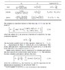
By using the attached formulation, I got the root of the function lambda is 0.03303492.
However, I increased the time, and the temperature in the unexposed wall was reduced. and when I change the time to 1 (one), the value shows almost like the T imposed, which is 100. Kind of the opposite way, Kindly any body help me with that. I also attached the script below

from scipy.optimize import fsolve
import numpy as np

def xtanxmbi(x, Bi):
    # tan = np.tan(x*np.pi/180)
    # return np.arctan(tan)*Bi-x
    # return (1/np.tan(x))*Bi-x
    return (np.cos(x)/np.sin(x))*Bi-x

# W = 1
# H = 0.1
L = 2.5 / 1000
qin = 0
Tinf = 100
Tini = 20
rhocp = 7850 * 460
k = 45.8
h = 20
alpha = k / rhocp
t = 360
Fo = alpha * t / (L**2)
print(f"The Fo is = {Fo}")
N = 6
n = 6
Bi = h * L / k
theta = np.zeros((n, N))
x0 = np.arange(n) * np.pi + 0.3
ans = fsolve(xtanxmbi, x0=x0, args=(Bi), full_output=True)
if ans[2] != 1:
    print("error solving roots of transcendental equation")
roots = ans[0]
Bi5 = Bi
print(f"Bi = {Bi5} , {roots}")

for i in np.arange(n):
    An = 2* np.sin(roots[I]) / (roots[I]+np.sin(roots[I])*np.cos(roots[I]))
    print(f"An = {An}")
    x = 1
    theta[I] = An * np.exp((-roots[I] ** 2 )* Fo) * np.cos(roots[I] * x)
    print(f"value of theta = {theta}")
    print(type(theta))
# Cn_0 = 4.0 * np.sin(roots[0]) / (2.0 * roots[0] + np.sin(2.0 * roots[0]))
# print(f"value of Cn is ={Cn_0}")
# theta_0 = Cn_0 * np.exp(-roots[0] ** 2 * Fo) * np.cos(roots[0] * x)
# print(f"value of theta is ={theta_0}")
sum_theta = theta[0, 0]
# print(sum_theta)

T = Tini + (Tinf - Tini) * sum_theta
print(f"value T={T}")

[/I][/I][/I][/I][/I][/I][/I]

 

[Chestermiller]

Please provide a diagram.

 

[Chestermiller]

The units of Cp are incorrect

 

[Chestermiller]

As an engineer, my approach to this is entirely different, and I actually get a simple accurate answer. Looking at the time scale for flattening of the temperature within the wall $L^2/\alpha$, I conclude that this time scale is only a few seconds, compared to the time scale for the thermal inertia of the wall to respond to the outside heat transfer $\tau = \rho C_p L/h$, which is on the order of 900 sec. So it is valid to use an lumped parameter model for the slab, with the temperature profile within the slab treated as uniform. For this description, the temperature is a function only of time, given by $$T=100-(100-20)e^{-t/\tau}$$At 360 seconds, this gives a temperature of about 46 C.