Master1022
- 590
- 116
- TL;DR
- Question about the derivation of the controllable canonical form for state space systems
Hi,
I was recently being taught a control theory course and was going through a 'derivation' of the controllable canonical form. I have a question about a certain step in the process.
Question: Why does the coefficient ## b_0 ## in front of the ## u(t) ## mean that the output ## y(t) = b_0 y_1 (t) ##? I understand that this probably doesn't make sense at the moment, but below are pictures of the derivation. The last two pictures show the introduction of these ##b_0## and ## b_1 ## constants and I am not sure why including ## b_0 u(t) ## leads to us scaling the output ## y(t) ## by ## b_0 ##? ## u(t) ## is only one component of the expression for ## \frac{d^n y}{dt^n} ##.
In my mind, it is almost as if we have: ## y = c_1 x_1 + c_2 x_2 + x_3 ##. Then, we change the coefficient of ## x_3 ## to ## c_3 ## and are now claiming that ## y ## is scaled by ## c_3 ##. I think I am missing something.
Any help is greatly appreciated.
Method:
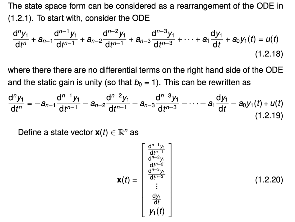
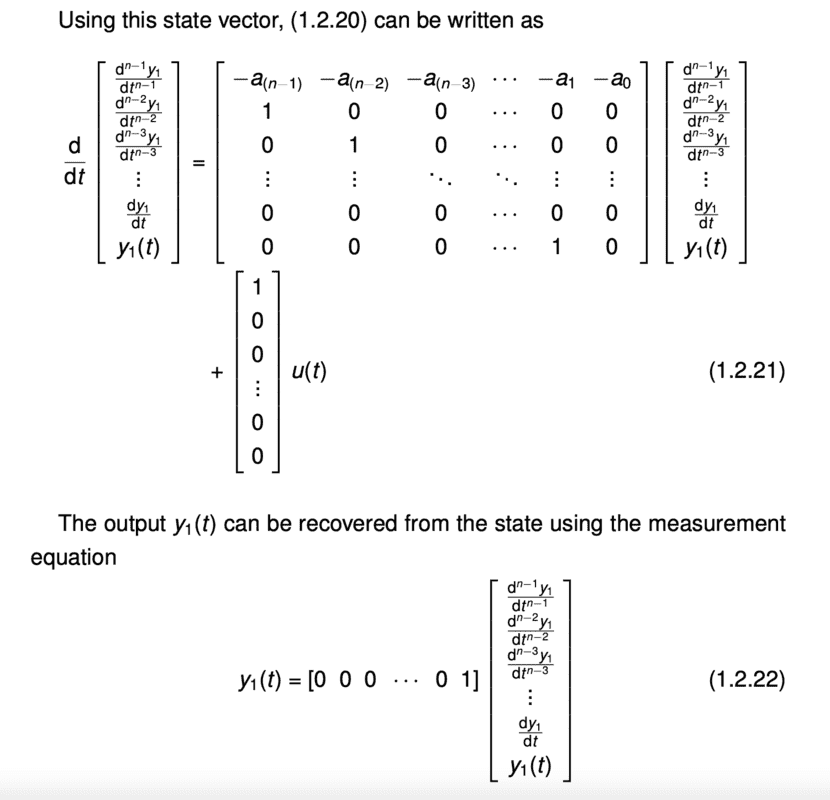
This is where ## b_0 ## is introduced.
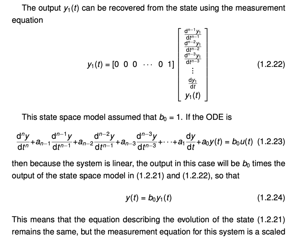
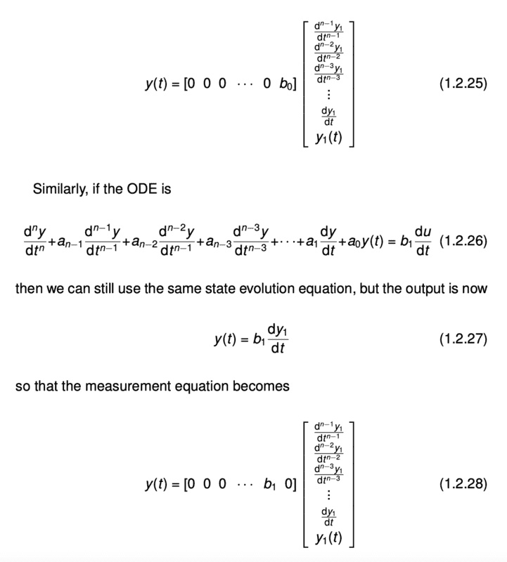
I was recently being taught a control theory course and was going through a 'derivation' of the controllable canonical form. I have a question about a certain step in the process.
Question: Why does the coefficient ## b_0 ## in front of the ## u(t) ## mean that the output ## y(t) = b_0 y_1 (t) ##? I understand that this probably doesn't make sense at the moment, but below are pictures of the derivation. The last two pictures show the introduction of these ##b_0## and ## b_1 ## constants and I am not sure why including ## b_0 u(t) ## leads to us scaling the output ## y(t) ## by ## b_0 ##? ## u(t) ## is only one component of the expression for ## \frac{d^n y}{dt^n} ##.
In my mind, it is almost as if we have: ## y = c_1 x_1 + c_2 x_2 + x_3 ##. Then, we change the coefficient of ## x_3 ## to ## c_3 ## and are now claiming that ## y ## is scaled by ## c_3 ##. I think I am missing something.
Any help is greatly appreciated.
Method:
This is where ## b_0 ## is introduced.