Ladder-like bandpass filter theoretical analysis problem

In summary, you have created a cascade of identical HP and LP filters, and you are not matching their impedance.
  • #1
room_
11
0
TL;DR Summary
I find the transfer function of the band-pass filter and its inverse Laplace yields not an impulse response but transient one.
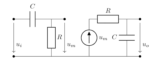
I consider the band-pass filter of the following configuration (the ##u_m## is a voltage controlled voltage source):
1589830476226.png
The transfer function is
$$K_1(p)=\hat{U}_o(p) = \frac{p}{RC(p+1/RC)^2} = \frac{\omega_c p}{(p+\omega_c)^2}, \quad \omega_c=\frac{1}{RC}.\qquad (1)$$

Now I connect ##n## such filters in a row (using the ##u_o## of a previous one as a source for next's ##u_i## by means of the controlled voltage source), which means that the transfer function becomes
$$ K_n(p)=\frac{\omega_c^{n}p^{n}}{(p+\omega_c)^{2n}}. \qquad (2)$$
To compensate the decrease in voltage on cutoff (same as center here) frequency ##\omega_c## I add ##2^n## factor (since every filter decreases voltage twice):
$$ K_n(p)=\frac{2^n\omega_c^{n}p^{n}}{(p+\omega_c)^{2n}}.\qquad (3)$$
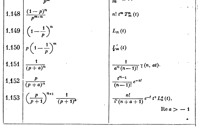
In some operational calculus handbook (russian one, not sure if it's reasonable to link) I find
1589837348326.png
I assume there is no problem in substituting ##n## for ##2n## in ##1.152##:
$$\hat{S}(p)=\frac{p}{(p+a)^{2n}}\div \frac{t^{2n-1}}{(2n-1)!}e^{-at}=s(t). \qquad(4) $$
Note that all of the derivatives of ##s(t)## up to ##n-2## order are equal to zero at ##t=0##. Finally I get the impulse response (using previous statement)
$$p^{n-1}2^n \omega_c^n \frac{p}{(p+\omega_c)^{2n}}-\sum_{k=0}^{n-2}p^{n-2-k} s^{(k)}(0) \div \frac{d^{n-1}}{dt^{n-1}} s(t),\qquad (5) \\
K_n(p)= \frac{2^n \omega_c^np^n}{(p+\omega_c)^{2n}}\div \frac{2^n\omega_c^n}{(2n-1)!}\frac{d^{n-1}}{dt^{n-1}}(e^{-\omega_c t}t^{2n-1})=k_n(t).\qquad (6)$$
I don't know why, but ##(6)## yields transient response (if to leave out the ##2^n## factor) ##h_n(t)## for my filter. i.e.
$$h_n(t)=\frac{\omega_c^n}{(2n-1)!}\frac{d^{n-1}}{dt^{n-1}}(e^{-\omega_c t}t^{2n-1}), \qquad (7)$$
although it is known that ##k(t)=\dfrac{d}{dt}h(t)##.
It is clear at least for ##n=1##. I plotted it in Matlab for ##n<30## (because Matlab refuses to calculate derivative of a higher order) and it looks
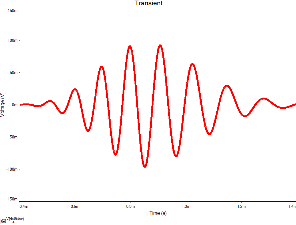
the way the simulation in NI Multisim gives. Here's ##n=49## (in Multisim):
1589834732954.png
It's predecessors (smaller ##n##'s) look alike, just having "less waves". WolframAlpha inverse Laplace suggestion (check my previous post) for transient response works for ##n\approx30\div50##, which is not satisfying. I assume there's something wrong with my reasoning, so I ask you to help me to find the mistake. Been struggling with it for a while and I need a fresh look on the problem. Thank you in advance.
 
Engineering news on Phys.org
  • #2
Cascading identical filter sections is not normally done because it increases the in-band ripple, while cascading odd/even order filters, or frequency staggering filters will flatten the pass-band.

Is the transient seen the tuned peak of the cascaded identical sections, or the Gibb's phenomenon.
https://en.wikipedia.org/wiki/Gibbs_phenomenon

A filter can attenuate unwanted energy by reflection from the input, or by internal resistive dissipation. You need to pay careful attention to the impedance matching of the filter sections.

That matching cannot be satisfied between stages if the match is one dimensional, such as a voltage buffer with infinite input impedance and zero output impedance.
 
  • Like
  • Informative
Likes dlgoff, room_ and berkeman
  • #3
Baluncore said:
Is the transient seen the tuned peak of the cascaded identical sections, or the Gibb's phenomenon.
What it has to do with the Gibbs phenomenon in this case? I may be missing the point.
Baluncore said:
You need to pay careful attention to the impedance matching of the filter sections.

That matching cannot be satisfied between stages if the match is one dimensional, such as a voltage buffer with infinite input impedance and zero output impedance.
Would you please describe it in a little simpler manner? I don't understand why the matching cannot be satisfied and what does that mean. I don't work with real network here, I only play around with the ideal simulation and I wish to understand the process behind. Thank you for response.
 
  • #4
room_ said:
What it has to do with the Gibbs phenomenon in this case? I may be missing the point.
Gibbs phenomenon is seen when an infinite expansion is terminated at a finite term, or all harmonics above a certain frequency are heavily attenuated. The limitations of Matlab 30, or Multisym 49, indicates that Gibbs phenomenon is a possibility.

You are isolating each HP and each LP section by a voltage follower, so no impedance matching is involved.
Examining the red trace impulse response. The oscillation has a period of about 0.1m sec which is a frequency of 10 kHz. That tells me the R and C were specified as something other than unity.
The risetime of the envelope is about 4 cycles which tells me the Q of the cascade is about 4.
The group delay of 49 stages is about 0.85 msec, or 17.34 usec per stage.
I assume it is stimulated by a narrow impulse at time = 0.

You have synthesised a narrow band delay line.
The transient response is very close to what I would expect for the cascade of 49 modules.

Why do you not trust your model?
Was the stimulus a unit area impulse?
Can you tell me what values of R and C you used to generate the red trace transient response?
 
  • #5
Baluncore said:
The limitations of Matlab 30, or Multisym 49, indicates that Gibbs phenomenon is a possibility.
There was no limitation seen in Multisim, 49 is just an example, yet it was the biggest I went because it's quite hard for my PC to run simulation with that many filters. Speaking of Matlab, I think it's the "large numbers" limitation, since it is clear that all of derivatives exist and can be calculated directly.
Baluncore said:
I assume it is stimulated by a narrow impulse at time = 0.
Baluncore said:
Was the stimulus a unit area impulse?
I seek for transient response, so it was stimulated by Heaviside step function ##1(t)##
Baluncore said:
Why do you not trust your model?
My reasoning brings me to the fact that transfer function yields transient response (instead of impulse one), which indicates that either my reasoning is wrong, or the inverse Laplace transform table has a mistake.
Baluncore said:
Can you tell me what values of R and C you used to generate the red trace transient response?
Here's one cascade
1589912785187.png
 
  • #6
Simulation of 49 cascaded modules with LTspice agrees with your transient response.
Stimulation is a 1 volt step at time = 0. PARAM Cx=80n Rx=220R
Zoom in on response shows; Centre frequency = 9.040 kHz Group delay = 862.70 usec
Bandwidth between -3.01dB points = 2.1642 kHz

Cascade49.png


Transient49.png

Transient response; Total computation elapsed time = 0.341 seconds.

Transfer function; Total computation elapsed time = 0.198 seconds.
3dBnose49.png


Bode49.png
 
Last edited:
  • Like
Likes room_
  • #7
Baluncore said:
Simulation of 49 cascaded modules with LTspice agrees with your transient response.
How many filters can you add more? Is it possible to go for ##n=100,200##? It would be very interesting to see.
 
  • #8
For 100 modules it produces the transfer function in 0.374 seconds.
-1.3k dB at 10 kHz; -1.5k dB at 100 kHz.
-535.7u dB at Fo, so there is still some dynamic range.

The transient response takes 0.469 seconds to compute.
Transient100.png
 
  • #9
The transient response of 200 modules takes 0.769 seconds to compute.
Transient200.png
 
  • Wow
Likes room_
  • #10
This is getting silly. The graphical interface is now a bit slow.
The transient response for 400 modules takes 4.497 seconds to compute.
Cascade 400.png
 
  • Like
Likes room_
  • #11
Baluncore said:
This is now getting silly. The graphical interface is now a bit slow.
The transient response for 400 modules takes 4.497 seconds to compute.
View attachment 263113
It is clear now how the impulse behaves with the growth of ##n##. What would you recommend to try to compute ##(7)## formula in the post? As previously mentioned, Matlab spits out 0 for ##n>30##, but I really want to see if it's the same as your results for ##n=100,200,400##.
 
  • #12
room_ said:
What would you recommend to try to compute (7)(7)(7) formula in the post?
You arrived at the transient stage by mathematics and questioned if it was correct. If a mathematician had followed you, they might have fallen into the same hole(s). I arrived at the same transient stage via a different path, which to some extent confirms your result.

It appears to me that your Hn(t), eqn 7, would need to be evaluated the hard way. Not being a mathematician leaves me at a disadvantage so I would need to go study for a day or two before writing the code. If you could expand eqn 7 into a computational process, that would help.
 
  • #13
Baluncore said:
If you could expand eqn 7 into a computational process, that would help.
##(7)## can be expressed in terms of generalized Laguerre polynomials (here I add ##2^n## factor)
$$h_n(t)= 2^n\omega_c^n \frac{(n-1)!}{(2n-1)!}t^n e^{-\omega_c t} L_{n-1}^{(n)}(t),$$
I guess there are procedures for computing them, hope it helps.
 
  • #14
room_ said:
$$h_n(t)= 2^n\omega_c^n \frac{(n-1)!}{(2n-1)!}t^n e^{-\omega_c t} L_{n-1}^{(n)}(t),$$
Sorry, the formula has to be
$$h_n(t)= 2^n\omega_c^n \frac{(n-1)!}{(2n-1)!}t^n e^{-\omega_c t} L_{n-1}^{(n)}(\omega_c t),$$
 
  • #15
The following paper refers to a Fortran 90 module (LaguerrePol)
Where can I find a copy of the source code for that module?

Efficient computation of Laguerre polynomials. A. Gil, J. Segura, N. M. Temme. 2016
https://arxiv.org/abs/1609.00829
 
  • #16
Baluncore said:
The following paper refers to a Fortran 90 module (LaguerrePol)
Where can I find a copy of the source code for that module?

Efficient computation of Laguerre polynomials. A. Gil, J. Segura, N. M. Temme. 2016
https://arxiv.org/abs/1609.00829
Files are at:
https://md-datasets-cache-zipfiles-prod.s3.eu-west-1.amazonaws.com/3jkk659cn8-1.zip
(only had to dig about 6 layers deep for that one! :rolleyes:)

The article with live links for the references is at:
https://kundoc.com/pdf-efficient-computation-of-laguerre-polynomials.html

Cheers,
Tom
 
  • Like
Likes room_ and Baluncore
  • #17
Baluncore said:
The following paper refers to a Fortran 90 module (LaguerrePol)
Where can I find a copy of the source code for that module?

Efficient computation of Laguerre polynomials. A. Gil, J. Segura, N. M. Temme. 2016
https://arxiv.org/abs/1609.00829
As the paper present, this algorithm works for large ##n## and small ##\alpha##, whereas in this case we have ##(\alpha) = (n) > n-1##. They suggest that the input parameters are ##-1\leq \alpha \leq 5, \ n\geq 0##, which allows us to compute as much as ##L_{4}^{5}(\omega_c t)##. This result can be easily obtained using Matlab, or just explicit differentiation.
Here's some other fortran library for computing Laguerre polynomials, haven't checked its efficiency yet because I don't know how to properly install libraries for fortran. It is also unknown whether it works for large ##n## and ##\alpha##.

Also, the problem stated in the first message in this thread is now solved. For anyone interested: the table I presented has a mistake - ##1.152##'s original should be the one for ##1.151##, therefore the formula obtained is correct and the only thing left is to come up with a way to compute Laguerre polynomials (or ##(7)##) to see whether the result is satisfying.
 
  • #18
I wrote LTspice subcircuits, nested with local parameters for the model. By eliminating the analysis of graphical connections I took the number of stages cascaded to 5000, (without hitting a limit). The result is what is expected. As the bandwidth is reduced, frequencies on either side of the pass-band that would sum destructively to cancel the centre frequency, become closer in frequency, so more cycles at the centre frequency are seen over a longer period. Also, the available step energy falling in the narrower bandwidth is reduced, so the output amplitude falls.
cascade5000.png


LTspice5000.png
 
  • Like
Likes room_
  • #19
@room_
What do you consider to be large n?

n, (2^n) * (n-1)! / (2n-1)!
1, 2.00000000000000000
2, 0.66666666666666667
3, 0.13333333333333333
4, 0.01904761904761905
5, 0.00211640211640212
6, 0.00019240019240019
7, 0.00001480001480001
8, 0.00000098666765333
9, 0.00000005803927373
10, 0.00000000305469862
11, 0.00000000014546184
12, 0.00000000000632443
13, 0.00000000000025298
14, 0.00000000000000937
15, 0.00000000000000032
 
  • #20
Baluncore said:
What do you consider to be large n?
##n>>1##, ##n\sim100## and above I guess can be considered as large.
 
  • #21
Here are later versions of the files used for post #18
 

Attachments

  • subckt2.asc.txt
    2.3 KB · Views: 123
  • subckt2.plt.txt
    625 bytes · Views: 140

1. What is a ladder-like bandpass filter?

A ladder-like bandpass filter is a type of electronic filter that allows a specific range of frequencies to pass through while blocking all others. It is composed of a series of inductors and capacitors arranged in a ladder-like structure.

2. How does a ladder-like bandpass filter work?

A ladder-like bandpass filter works by creating a resonant circuit that only allows a specific range of frequencies to pass through. The inductors and capacitors in the circuit work together to create a peak in the frequency response curve, allowing the desired frequencies to pass through while attenuating all others.

3. What is the theoretical analysis problem associated with ladder-like bandpass filters?

The theoretical analysis problem with ladder-like bandpass filters is that their performance may deviate from the expected ideal behavior due to various factors such as component tolerances, parasitic effects, and non-ideal behavior of the components.

4. How is the theoretical analysis of ladder-like bandpass filters performed?

The theoretical analysis of ladder-like bandpass filters is typically performed using mathematical equations and circuit analysis techniques. This involves calculating the filter's transfer function, frequency response, and other parameters to determine its performance under ideal conditions.

5. What are some common applications of ladder-like bandpass filters?

Ladder-like bandpass filters are commonly used in electronic devices and systems to isolate specific frequencies and remove unwanted noise. They are also used in communication systems, audio equipment, and instrumentation to improve signal quality and selectivity.

Similar threads

Replies
4
Views
184
Replies
2
Views
1K
  • Advanced Physics Homework Help
Replies
6
Views
1K
  • Calculus and Beyond Homework Help
Replies
3
Views
482
  • Classical Physics
Replies
4
Views
675
Replies
16
Views
1K
Replies
1
Views
503
  • Math Proof Training and Practice
2
Replies
48
Views
9K
  • Math Proof Training and Practice
2
Replies
61
Views
9K
  • Math Proof Training and Practice
3
Replies
86
Views
9K
Back
Top