I Looking For Help Understanding Bell's Theorem, Hidden Variables & QM

[Lynch101]

TL;DR Summary

A few questions on Bell's inequality, which might serve as a means for helping me better understand Bell's Theorem, Hidden Variables & QM.

I was revisiting @DrChinese 's Bell's Theorem with Easy Math which sparked a few questions, which I am hoping might offer a potential path to a deeper understanding of Bell's Theorem and Quantum Mechanics (QM) in general.

The explanation uses light polarisation experiments to explain how we arrive at Bell's inequality.

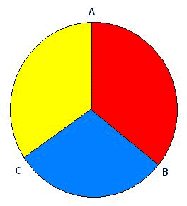
We can't explain why a photon's polarization takes on the values it does at angle settings A, B and C. But we can measure it after the fact with a polarizer at one setting, and in some cases we can predict it for one setting in advance. The colors match up with the columns in Table 1 below. (By convention, the 0 degrees alignment corresponds to straight up.)

ASSUME that a photon has 3 simultaneously real Hidden Variables A, B and C at the angles 0 degrees, 120 degrees and 240 degrees per the diagram above. These 3 Hidden Variables, if they exist, would correspond to simultaneous elements of reality associated with the photon's measurable polarization attributes at measurement settings A, B and C.
...
[W]e are simply saying that the answers to the 3 questions "What is the polarization of a photon at: 0, 120 and 240 degrees?" exist independently of actually seeing them. If a photon has definite simultaneous values for these 3 polarization settings, then they must correspond to the 8 cases ([1]...[8]) presented in Table 1 below. So our first assumption is that reality is independent of observation, and we will check and see if that assumption holds up.

There are only three angle pairs to consider in the above: A and B (we'll call this [AB]); B and C (we'll call this [BC]); and lastly A and C (we'll call this [AC]). If A and B yielded the same values (either both + or both -), then [AB]=matched and we will call this a "1". If A and B yielded different values (one a + and the other a -), then [AB]=unmatched and we will call this a "0". Ditto for [BC] and [AC]. If you consider all of the permutations of what A, B and C can be, you come up with the following table:

(Emphasis mine)

It is pretty obvious from the table above that no matter which of the 8 scenarios which actually occur (and we have no control over this), the average likelihood of seeing a match for any pair must be at least .333
...
We don't know whether [Cases [1] and [8]] happen very often, but you can see that for any case the likelihood of a match is either 1/3 or 3/3). Thus you never get a rate less than 1/3 as long as you sample [AB], [BC] and [AC] evenly.
...
The fact that the matches should occur greater than or equal to 1/3 of the time is called Bell's Inequality.
...
Bell also noticed that QM predicts that the actual value will be .250, which is LESS than the "Hidden Variables" predicted value of at least .333
...
If [the experimental tests] are NOT in accordance with the .333 prediction, then our initial assumption above - that A, B and C exist simultaneously - must be WRONG.
...
Experiments support the predictions of QM.

When it says above to "assume that a photon has 3 simultaneously real Hidden Variables (HV) A, B and C [at the angles]" does this only apply to Hidden variables theories with these specific characteristics? Is it possible to have a HV theory which doesn't have these 3 simultaneously real Hidden Variables.

There is probably some basic answer to this, but in trying to think more about Bell's theorem, I was wondering if it would be possible that the photons are simply polarised North and South, where the line of polarisation (the axis?) would be the hidden variable and can take any orientation within 360 degrees? I was thinking that this would mean that any photon would have a probability 0.5 of passing a polarisation filter. For any pair of particles, there would be a probability of ≥0.25 of both photons passing through their respective filters.

F = fails to pass filter
P = passes filter
P/F = photon 1 passes/photon 2 fails
Pass = both pass their respective filters.There is probably lots wrong in that, but that is where my thinking has taken me, so any help to point out where I've gone wrong or gaps in my understanding would be greatly appreciated.

 

[DrChinese]

The explanation uses light polarisation experiments to explain how we arrive at Bell's inequality.
View attachment 334611

(Emphasis mine)

View attachment 334610
1. When it says above to "assume that a photon has 3 simultaneously real Hidden Variables (HV) A, B and C [at the angles]" does this only apply to Hidden variables theories with these specific characteristics? Is it possible to have a HV theory which doesn't have these 3 simultaneously real Hidden Variables.

2. There is probably some basic answer to this, but in trying to think more about Bell's theorem, I was wondering if it would be possible that the photons are simply polarised North and South, where the line of polarisation (the axis?) would be the hidden variable and can take any orientation within 360 degrees? I was thinking that this would mean that any photon would have a probability 0.5 of passing a polarisation filter. For any pair of particles, there would be a probability of ≥0.25 of both photons passing through their respective filters.

View attachment 334751
F = fails to pass filter
P = passes filter
P/F = photon 1 passes/photon 2 fails
Pass = both pass their respective filters.

1. This point has been debated by many, but the essential answer is: No, it is not possible that there can be a Hidden Variable theory that does not have "simultaneously real" values (answers to polarization measurements) for 3 or more (and possibly infinite) angles.

You can see this is the case from several different perspectives. From the theoretical side: This is the critical assumption in the Bell argument. He actually calls the angle settings a, b and c. See Bell (1964) after his formula (14). This is in response to the earlier and important EPR (1935) paper, which made a similar assumption. Their conclusion, which rested on this assumption, was that QM was not complete. They believed their assumption so obvious, that any other view was unreasonable.

"Indeed, one would not arrive at our conclusion if one insisted that two or more physical quantities can be regarded as simultaneous elements of reality only when they can be simultaneously measured or predicted. On this point of' view, since either one or the other, but not both simultaneously, of the quantities P and Q can be predicted, they are not simultaneously real. This makes the reality of P and Q depend upon the process of measurement carried out on the first system, which does, not disturb the second system in any way. No reasonable definition of reality could be expected to permit this."

Could there be other definitions of HVs that lack this assumption*? It would be hard, considering this is precisely the definition of a realistic theory in the first place. Moreover, from the practical side: they already knew that QM would predict perfect correlations if both Alice and Bob both measured P (or both Q - whatever they choose either to be). If there are perfect correlations, then this implies that the result must actually be predetermined.2. Hopefully you can now see the biggest problem with your hypothesis. That being on your chart. in the columns marked A/A, B/B and CC: There will be no F/P or P/F outcomes at all. So the statistics will be a mixture of F/F (50%) and P/P (the other 50%).

Note that in actual Bell experiments, a Polarizing Beam Splitter (PBS) is normally used rather than a Polarizer. That way you actually detect all photons (in the ideal case).*They of course also assumed that Alice's outcome would be independent (separable) from Bob's outcome (which is the Locality assumption). There are HV theories which do not include the Locality assumption.

 

[Lynch101]

1. This point has been debated by many, but the essential answer is: No, it is not possible that there can be a Hidden Variable theory that does not have "simultaneously real" values (answers to polarization measurements) for 3 or more (and possibly infinite) angles.

Ah yes, of course! My bad, the idea of HVs is that it's already "programmed" in advance whether they will pass the filters. I was more focused on trying to see if there was a way to get a HV model to match the predictions of QM, which made me overlook that particular point.

Thanks for the clarification.

 

[Lynch101]

Am I right in saying that we're also interested in the cases where the outcome is the same, not just where both pass?

 

[Lynch101]

This is a very basic question, and I would anticipate the answer, but I just want to ask for the sake of certainty.

In practice, does the statistical analysis of the statistical sample of experimental observations select for equal numbers of the possible detector combinations? That is, in terms of @DrChinese's explanation, does it select for an equal ratio of AB:BC:AC?

 

[PeterDonis]

does the statistical analysis of the statistical sample of experimental observations select for equal numbers of the possible detector combinations?

I don't know what you mean by "select for". The statistical analysis will tell you what proportion of the observations fall into each category.

 

[Nugatory]

In practice, does the statistical analysis of the statistical sample of experimental observations select for equal numbers of the possible detector combinations?

You may be describing what is called the “fair sampling loophole” - if some configurations of the hidden variables are more likely to go undetected in some detector configurations than others it is possible to find violations of the inequalities. This possibility has always been met with some skepticism because no one could propose a convincing (as opposed to a possible but contrived sort of devil’s advocate) model in which that would happen, but still the possibility existed.

However, this loophole was decisively closed by an experiment done a few years back.
I’ll post the link in a while if no one beats me to it.

 

[DrChinese]

You may be describing what is called the “fair sampling loophole” - if some configurations of the hidden variables are more likely to go undetected in some detector configurations than others it is possible to find violations of the inequalities. This possibility has always been met with some skepticism because no one could propose a convincing (as opposed to a possible but contrived sort of devil’s advocate) model in which that would happen, but still the possibility existed.

However, this loophole was decisively by an experiment done a few years back.
I’ll post the link in a while if no one beats me to it.

Here’s a good one without the fair sampling loophole :

https://arxiv.org/abs/1508.05949

 

[Nugatory]

Here’s a good one without the fair sampling loophole :

https://arxiv.org/abs/1508.05949

Yes, that's it - thanks.

 

[Lynch101]

Cheers, I'll check out that paper.

 

[Lynch101]

Are there tests of QT which don't randomly vary the detector settings? As in, which test a statistical sample of only two different detector settings e.g. AB (as per Dr.C's) explanation above?

 

[Lynch101]

Are there tests of QT which don't randomly vary the detector settings? As in, which test a statistical sample of only two different detector settings e.g. AB (as per Dr.C's) explanation above?

It's probably a gap in my understanding with regard to principles of statistics, but I'm wondering if each pairing of filters is treated as a statistically independent trial?

 

[Nugatory]

Are there tests of QT which don't randomly vary the detector settings? As in, which test a statistical sample of only two different detector settings e.g. AB (as per Dr.C's) explanation above?

Almost all of them, possibly every one that was done before the discovery of Bell's theorem led to interest in correlations between results at different detector settings. It's such basic stuff that it was a lab exercise required of all physics majors when I was in college - and the point of the experiment was not to test QT but to test the proposition "Nugatory is competent to set up and operate lab equipment"

 

[Nugatory]

It's probably a gap in my understanding with regard to principles of statistics, but I'm wondering if each pairing of filters is treated as a statistically independent trial?

Each entangled pair is treated as a separate trial, statistically independent of the previous and successive one. This is an assumption, but it is both reasonable and born out by observation of the statistical distribution of the behavior of the particle source.

Nonetheless it is an assumption. If you pull on this string you will eventually arrive at the only "loophole" that cannot be eliminated: superdeterminism. Search this forum for previous discussions of the idea - it is both irrefutable and an intellectual dead end.

 

[Lynch101]

Each entangled pair is treated as a separate trial, statistically independent of the previous and successive one. This is an assumption, but it is both reasonable and born out by observation of the statistical distribution of the behavior of the particle source.

Nonetheless it is an assumption. If you pull on this string you will eventually arrive at the only "loophole" that cannot be eliminated: superdeterminism. Search this forum for previous discussions of the idea - it is both irrefutable and an intellectual dead end.

I'm wondering about the independence of the filter orientations, as opposed to the entangled pairings. I know both of those are assumed to be statistically independent of each other, but I'm wondering about the independence of the filter settings with respect to each other (if that makes sense) - like how individual trials of rolling 2 dice are all independent of each other.

To clarify what I'm wondering about - and it's probably just that I'm reading it incorrectly or am missing a basic principle: is the likelihood of a match for each individual pair of filter settings not ≥ 0.25, if we don't know how often cases [1] and [8] occur?

From Dr.Ch's explanation:

Cases [1] and [8] actually always yield matches (3/3 or 100% of the time). We don't know whether these particular cases happen very often, but you can see that for any case the likelihood of a match is either...

 

[PeterDonis]

I'm wondering about the independence of the filter orientations, as opposed to the entangled pairings. I know both of those are assumed to be statistically independent of each other, but I'm wondering about the independence of the filter settings with respect to each other

We've had this discussion in previous threads of yours. The lack of statistical independence here is basically superdeterminism. There's no point in rehashing superdeterminism again here; as @Nugatory has said, it's already been discussed plenty in previous PF threads and the discussions lead nowhere.

 

[Lynch101]

We've had this discussion in previous threads of yours. The lack of statistical independence here is basically superdeterminism. There's no point in rehashing superdeterminism again here; as @Nugatory has said, it's already been discussed plenty in previous PF threads and the discussions lead nowhere.

I'm thinking along different lines this time, in line with what I, probably mistakenly, understand statistical independence to imply.

I was thinking that statistical independence of the choice of filter settings* would imply treating them as independent probabilistic events.

*Independent of other trials (of filter setting choices) as well as independent of the preparation of the photon pairs.

 

[PeterDonis]

I'm thinking along different lines this time

Not really.

I was thinking that statistical independence of the choice of filter settings* would imply treating them as independent probabilistic events.

Which is what superdeterminism denies.

 

[Lynch101]

Not really.Which is what superdeterminism denies.

In this case I'm not trying to deny it, rather affirming it - at least as far as my understanding extends.

 

[PeterDonis]

In this case I'm not trying to deny it, rather affirming it - at least as far as my understanding extends.

Which still leaves the discussion going nowhere. So you affirm superdeterminism: then what?

 

[Lynch101]

Which still leaves the discussion going nowhere. So you affirm superdeterminism: then what?

No, what I'm asking here would deny Superdeterminism (afaik).

I'm asking, if each filter combination is treated as a statistically independent event* (denial of Superdeterminism) would the probability of matching outcomes not be ≥0.25?

*Independent from other choices of filter combination as well as from particle preparation (denial of SD).

Again, I'm probably missing some nuance.

 

[PeterDonis]

if each filter combination is treated as a statistically independent event* (denial of Superdeterminism) would the probability of matching outcomes not be ≥0.25?

No, because superdeterminism is not the only possible interpretation of QM. All we really know is that QM correctly predicts the probability of matching outcomes that we actually observe, and that those probabilities violate the Bell inequalities or their equivalents. We don't know why that is: superdeterminism is just one possible "why".

 

[PeterDonis]

if each filter combination is treated as a statistically independent event

Note, btw, that we can do statistical tests on the filter combinations, to verify that they at least appear to be statistically independent. Superdeterminism has to claim that that appearance is in fact invalid: that there is a connection between them "behind the scenes", it's just set up in exactly the right way to mislead us into thinking the combinations are statistically independent, when they actually aren't.

 

[Lynch101]

Note, btw, that we can do statistical tests on the filter combinations, to verify that they at least appear to be statistically independent. Superdeterminism has to claim that that appearance is in fact invalid: that there is a connection between them "behind the scenes", it's just set up in exactly the right way to mislead us into thinking the combinations are statistically independent, when they actually aren't.

Sorry, I initially didn't understand what Superdeterminism had to do with it. I thought what I was asking implied the opposite.

I was thinking that treating each filter pairing as a statistically independent event was upholding statistical independence, but it doesn't uphold statistical independence of the filters and particle pairings.

 

[Lynch101]

Apologies, when I try to develop a better understanding of ideas I usually go back and forth with them and try to look at them from different perspectives. I sometimes get stuck on certain questions which are often quite basic. This is probably another pretty basic question.

I'm wondering what the distinction is between what I was doing here (looking at filter settings as statistically independent from other settings):

And this:

I'm wondering why it isn't the same reasoning as I was using, just applied to pairs of photons?A related question: why do we not consider the entire possibility space? If we discount cases [1] & [8] because we don't know how often those cases occur, the probability of seeing matching pairs would be 6/24 or ≥0.25.

I'm probably making some basic mistake here. I was just thinking about an explanation which helped me understand the Monty Hall problem and I (tried) applying it here.

 

[PeterDonis]

Sorry, I initially didn't understand what Superdeterminism had to do with it. I thought what I was asking implied the opposite.

If you are explicitly denying superdeterminism, you need to explicitly say so. Just saying "statistical independence" isn't enough, since, as I noted, a superdeterminist would claim that such independence is only apparent (since we can test for it but we have no way of actually knowing for sure that our tests aren't being superdetermined).

I was thinking that treating each filter pairing as a statistically independent event was upholding statistical independence, but it doesn't uphold statistical independence of the filters and particle pairings.

This is correct, yes. To fully deny superdeterminism you have to explicitly deny all such "behind the scenes" connections.

 

[PeterDonis]

I was just thinking about an explanation which helped me understand the Monty Hall problem and I (tried) applying it here.

You can't. The Monty Hall problem is solvable by local hidden variables (the hidden variables are just what is actually behind the doors)--but Bell's Theorem and its equivalents prove that local hidden variables cannot explain our actual observations in cases like the experiment you are looking at here. That is the point of the chart showing the 8 possible combinations of results and the average correlations for each: no matter how you combine all of those, you can't get an average of 0.25--but when we actually run the experiment, we do get an average of 0.25! So no local hidden variable model can explain the actual results, because any local hidden variable model would end up producing a chart like the one you are looking at, which cannot possibly explain the actual results.

 

[DrChinese]

If we discount cases [1] & [8] because we don't know how often those cases occur, the probability of seeing matching pairs would be 6/24 or ≥0.25.

Your denominator is incorrect. If you discount cases [1] & [8], you have remaining 6x3=18 cases. The fraction is then 6/18, which is back to .333 (and well different that the quantum expectation of .25).

 

[Lynch101]

Your denominator is incorrect. If you discount cases [1] & [8], you have remaining 6x3=18 cases. The fraction is then 6/18, which is back to .333 (and well different that the quantum expectation of .25).

I was thinking to discount them, but not totally disregard them as possibilities. As in , they could still possibly occur, we just don't know how often, which would give rise to the "greater than" part of the inequality.

I was thinking that by doing so, to borrow a sentence in your explanation, "thus you never get a rate less than" 0.25.

if that makes any sense?

 

[Lynch101]

You can't. The Monty Hall problem is solvable by local hidden variables (the hidden variables are just what is actually behind the doors)--but Bell's Theorem and its equivalents prove that local hidden variables cannot explain our actual observations in cases like the experiment you are looking at here. That is the point of the chart showing the 8 possible combinations of results and the average correlations for each: no matter how you combine all of those, you can't get an average of 0.25--but when we actually run the experiment, we do get an average of 0.25! So no local hidden variable model can explain the actual results, because any local hidden variable model would end up producing a chart like the one you are looking at, which cannot possibly explain the actual results.

Sorry, what I meant was that, what helped me understand the Monty Hall problem was seeing the entire possibility space laid out.

I was looking at the possibility space in Dr C's explanation and wondering why we don't consider the entire possibility space.

Dr.C, for want of a better word, ignored the cases where each photon had hidden variables which would ensure it passed all 3 filters or the opposite, ensured it would fail all 3. The reason was that we aren't sure how often those instances occur.

His conclusion was that "thus you never get a rate less than 0.333"

I was looking at the possibility space and applying that reasoning. If we discount them (but allow for them to occur) you never get a rate less than 0.25. Assuming they occur occasionally, the probability of seeing matches across the statistical sample would be ≥0.25.

I assume I'm misconstruing something there, I'm just not sure what it is.

 

[Lynch101]

@DrChinese, just to try and clarify further.

My understanding of your statement that we don't know how often cases [1] & [8] occur either implies or allows for the possibility that they occur infrequently, which is why I am thinking we can discount them when calculating the minimum probability, but not exclude them from the possibility space.

 

[PeterDonis]

Dr.C, for want of a better word, ignored the cases where each photon had hidden variables which would ensure it passed all 3 filters or the opposite, ensured it would fail all 3.

I don't know what you're talking about. The table @DrChinese gave covers all possible combinations of results. No combinations are ignored. The case where all 3 filters are passed and the case where all 3 filters fail is included in the table.

It doesn't matter what other structure there is "underneath" that produces the results. The point is that no possible table of predetermined results can match the QM prediction.

Furthermore, this is true whether we ignore the "pass all 3" and "fail all 3" possibilities or not. Either way no possible table of results can match the QM prediction.

I think you have not grasped the actual argument @DrChinese has been describing.

 

[PeterDonis]

If we discount them (but allow for them to occur)

What does this even mean?

 

[Lynch101]

I don't know what you're talking about. The table @DrChinese gave covers all possible combinations of results. No combinations are ignored. The case where all 3 filters are passed and the case where all 3 filters fail is included in the table.

I can see where the average of 0.333 comes from, but it doesn't come from the average of the entire possibility space. While cases [1] and [8] are represented in the table, when it comes to calculating the average, they are ignored (which is what I mean when I say discounted). The reason given for this is because we don't know how often they occur.

Instead, the average for each row is taken, except for cases [1] and [8].

But, when I was asking about the case where we consider each column:

you immediately saw that this didn't treat the choice of filters as statistically independent of the particle pairs and therefore implied Superdeterminism. I didn't see it myself initially, but after thinking about, it I think I understand how you arrived at that conclusion.

That prompted me to wonder why taking the average of an individual row wasn't the same principle, just applied to particle pairs.

I was thinking that, for statistically independent events, we should consider the possibility space as a whole, as in this representation - where there are 24 possible outcomes:

This got me wondering, if we don't know how often cases [1] and [8] occur, it might be possible that they occur much less frequently than the other cases. It might be the case that in a given statistical sample they don't occur at all, while in other statistical samples they do occur.

If that were the case, the space of possible outcomes would still be 24 but the minimum number of matches we would expect to see would be 6/24 = 0.25. That is arrived at when we consider the other cases, which occur more frequently.

I was thinking that when we factor in cases [1] and [8] we would expect ≥0.25 matches.

It doesn't matter what other structure there is "underneath" that produces the results. The point is that no possible table of predetermined results can match the QM prediction.

Furthermore, this is true whether we ignore the "pass all 3" and "fail all 3" possibilities or not. Either way no possible table of results can match the QM prediction.

My thinking is that, if cases [1] * [8] ("pass all 3" and "fail all 3") occur much less frequently that the other cases i.e. there is not an equal chance of them occurring, then they would remain in the space of possibilities but (borrowing DrC's words) "you never get a rate less than" 0.25).

I think you have not grasped the actual argument @DrChinese has been describing.

I can see where the average of 0.333 comes from. My questions might be more to do with the application and interpretation of the statistics in general.

 

[Lynch101]

What does this even mean?

What I mean by that is, it's always a possibility that cases [1] & [8] occur, so we have to include them in our space of possible outcomes. However, because they are not as likely to occur as the other cases (with a possibility they don't occur in a given statistical sample), we don't count them when calculating the minimum expectation value (of matching outcomes).

Where they occur, they could give us a value ≥0.25.

 

[DrChinese]

@DrChinese, just to try and clarify further.

My understanding of your statement that we don't know how often cases [1] & [8] occur either implies or allows for the possibility that they occur infrequently, which is why I am thinking we can discount them when calculating the minimum probability, but not exclude them from the possibility space.

What I mean by that is, it's always a possibility that cases [1] & [8] occur, so we have to include them in our space of possible outcomes. However, because they are not as likely to occur as the other cases (with a possibility they don't occur in a given statistical sample), we don't count them when calculating the minimum expectation value (of matching outcomes).

Where they occur, they could give us a value ≥0.25.

Here are some relevant rules for calculating any statistical situations:

a) If you include the cases in the denominator, you must also include the associated data in the numerator.
b) You are free to change the weighting of the cases according to your own viewpoint or rationale. For example, while I might suggest all 8 cases are equally likely, you might reasonably argue that cases [1] and [8] are rare - so you weight them as 0%. You might even say case [2] is twice as likely as case [3]. Fine. However, that still leads us to exactly the same minimum of .333 - and not .250. There are no cases with a match % less than .333.

Next, consider this: you can even make up your own results for as many trials as you like, picking whatever cases you like. And unless you pick those cases knowing in advance which 2 measurement settings (of 3) you plan to use, you will never have an average less than .333.

 

[PeterDonis]

I can see where the average of 0.333 comes from, but it doesn't come from the average of the entire possibility space.

The average if you include rows 1 and 8 is even higher.

What I mean by that is, it's always a possibility that cases [1] & [8] occur, so we have to include them in our space of possible outcomes.

Ok.

However, because they are not as likely to occur as the other cases (with a possibility they don't occur in a given statistical sample), we don't count them when calculating the minimum expectation value (of matching outcomes).

Nonsense. Doing statistics doesn't mean ignoring things that are less likely. At most, it means weighting the different possibilities by likelihood. You can't just make up your own statistical methods.

Even leaving all that aside, as noted above, the average if you include rows 1 and 8, at any statistical weight whatever, is even higher than 0.333. So there is still no way to get an average of 0.25. So even if your objective is to calculate the minimum expectation value for the table, that would not imply ignoring rows 1 and 8 because they are less likely. It would at most imply ignoring rows 1 and 8 because they would just increase the average.

 

[Lynch101]

Here are some relevant rules for calculating any statistical situations:

a) If you include the cases in the denominator, you must also include the associated data in the numerator.
b) You are free to change the weighting of the cases according to your own viewpoint or rationale. For example, while I might suggest all 8 cases are equally likely, you might reasonably argue that cases [1] and [8] are rare - so you weight them as 0%. You might even say case [2] is twice as likely as case [3]. Fine. However, that still leads us to exactly the same minimum of .333 - and not .250. There are no cases with a match % less than .333.

Next, consider this: you can even make up your own results for as many trials as you like, picking whatever cases you like. And unless you pick those cases knowing in advance which 2 measurement settings (of 3) you plan to use, you will never have an average less than .333.

Cheers for this clarification. I was toying with the idea of weighting, but didn't have time to work through permutations.

I misinterpreted what you said in the explanation on your website, when you said about cases [1] and [8] that we don't know how often they occur which gave rise to the line of thinking of the past few posts.

Thinking through it further, obviously the ratio of matches to mismatches (without cases [1] & [8]) is 1:2 and given there must be some outcome of each trial, if cases [1] & [8] never occur the ratio of matches to mismatches for the statistical sample will have to be 1:2 (minimum number of matches being 1/3).Presumably it's not possible that instead of cases [1] & [8] being the case:
Photon 1: A+B+C+
Photon 2: A+B+C+

It was
Photon 1: A+B+C+
Photon 2: A-B-C-

Presumably there's either some experiment which has ruled this out, or it would it make any difference?

I've tried working it out on a spreadsheet, but as you may understand, I'm slow to trust my own analysis when it comes to statistics.

 

[Lynch101]

The average if you include rows 1 and 8 is even higher.

Yes, I was misinterpreting DrC's statement about not knowing how often cases [1] and [8] occur, but I've played around with it. I tried imagining a roulette wheel and weighting the different outcomes.

Nonsense. Doing statistics doesn't mean ignoring things that are less likely. At most, it means weighting the different possibilities by likelihood. You can't just make up your own statistical methods.

Hahaha, I wouldn't dream of it. Toying around with weighting helped me to grasp it.

Even leaving all that aside, as noted above, the average if you include rows 1 and 8, at any statistical weight whatever, is even higher than 0.333. So there is still no way to get an average of 0.25. So even if your objective is to calculate the minimum expectation value for the table, that would not imply ignoring rows 1 and 8 because they are less likely. It would at most imply ignoring rows 1 and 8 because they would just increase the average.

Thanks for taking the time to explain it.

 

[PeterDonis]

Presumably it's not possible that instead of cases [1] & [8] being the case:
Photon 1: A+B+C+
Photon 2: A+B+C+

It was
Photon 1: A+B+C+
Photon 2: A-B-C-

There is no "Photon 2" in the scenario @DrChinese described.

 

[Lynch101]

There is no "Photon 2" in the scenario @DrChinese described.

 

[Lynch101]

Ah, that would explain a lot.

I was thinking in terms of pairs of photons being sent to separate detectors . I thought there was an assumption that each photon has the same properties.

 

[PeterDonis]

I was thinking in terms of pairs of photons being sent to separate detectors . I thought there was an assumption that each photon has the same properties.

In the scenario @DrChinese described, a local hidden variable model is being tested. In that model, each individual photon has pre-determined values for all three measurements, A, B, and C. The model is tested by making measurements on a large number of identically prepared photons. But in each individual measurement, only one photon is measured.

 

[Lynch101]

In the scenario @DrChinese described, a local hidden variable model is being tested. In that model, each individual photon has pre-determined values for all three measurements, A, B, and C. The model is tested by making measurements on a large number of identically prepared photons. But in each individual measurement, only one photon is measured.

Thanks PD. I re-visited the statistics without re-reading the whole thing and had it in my head that it was photon pairs.

Thanks for taking the time to address my confused posts in this thread!

 

[Lynch101]

In the scenario @DrChinese described, a local hidden variable model is being tested. In that model, each individual photon has pre-determined values for all three measurements, A, B, and C. The model is tested by making measurements on a large number of identically prepared photons. But in each individual measurement, only one photon is measured.

Can that experimental set-up be used to test Bell's inequality?

I may again have misinterpreted DrC's explanation when he said

d. Bell anticipated that this result sounded good in theory, but needed more to make sense - because the above conclusion could not be tested......Using [...] entangled particles, it would be possible to measure 2 of the 3 settings mentioned above simultaneously, thus providing a way to differentiate between QM and Hidden Variables experimentally using Bell's Inequality

I may have been confusing it with this explanation, which is where the assumption of photon pairs may have come from:
DrPhysicsA - Bell's Inequality

 

[PeterDonis]

Can that experimental set-up be used to test Bell's inequality?

Not directly since only one photon is involved, not an entangled pair. But it can serve as a test of the QM prediction, which is for an average correlation of 0.25, and which, if enough runs are done, can be distinguished from the prediction of a local hidden variable model.

 

[Lynch101]

Not directly since only one photon is involved, not an entangled pair. But it can serve as a test of the QM prediction, which is for an average correlation of 0.25, and which, if enough runs are done, can be distinguished from the prediction of a local hidden variable model.

Ah cool. I was thinking that.

Cheers for the clarification.

 

[Lynch101]

There is no "Photon 2" in the scenario @DrChinese described.

Sorry, just going back to this. In tests of Bell's inequality, where entangled pairs of photons are used, would it be be possible that in cases [1] & [8] the two photons would have the following HVs:

Photon 1: A+B+C+
Photon 2: A-B-C-

or vice versa?

 

[PeterDonis]

In tests of Bell's inequality...

The table of possible values would be different, since there are two photons, not one. There would be 64 possible cases, not 8.

 

[Lynch101]

The table of possible values would be different, since there are two photons, not one. There would be 64 possible cases, not 8.

Would that be the case even if the photons were always identical except in cases [1] & [8]?